In this chapter we will be covering some of the key measures and relationships of a business operation. To help illustrate these concepts, we will consider the following simple business venture opportunity.
Suppose three students like spending time at the beach. They have pondered whether they could work and live at the beach during their summer break and learned that they could lease a small building by the beach with existing freezer capacity and apply for a local license to sell ice cream bars.
Most businesses sell something—either a physical commodity like an ice cream bar or a service like a car repair. In a modern economy, that sale is made in return for money or at least is evaluated in monetary terms. The total monetary value of the goods or services sold is called revenueThe total monetary value of the goods or services that a business sells..
Few businesses are able to sell something without incurring expenses to make the sale possible. The collective expenses incurred to generate revenue over a period of time, expressed in terms of monetary value, are the costThe collective expenses incurred to generate revenue over a period of time, expressed in terms of monetary value.. Some cost elements are related to the volume of sales; that is, as sales go up, the expenses go up. These costs are called variable costsExpenses that change as the the volume of sales changes.. The cost of raw materials used to make an item of clothing would be an example of a variable cost. Other costs are largely invariant to the volume of sales, at least within a certain range of sales volumes. These costs are called fixed costsExpenses that remain the same regardless of the volume of sales or that remain the same within a certain range of sales volumes.. The cost of a machine for cutting cloth to make an item of clothing would be a fixed cost.
Businesses are viable on a sustained basis only when the revenue generated by the business generally exceeds the cost incurred in operating the business. The difference between the revenue and cost (found by subtracting the cost from the revenue) is called the profitThe difference between revenue and cost when revenue exceeds the cost incurred in operating the business.. When costs exceed revenue, there is a negative profit, or lossThe difference between revenue and cost when the cost incurred in operating the business exceeds revenue..
The students in our simple venture realize they need to determine whether they can make a profit from a summer ice cream bar business. They met the person who operated an ice cream bar business in this building the previous summer. He told them last summer he charged $1.50 per ice cream bar and sold 36,000 ice cream bars. He said the cost of the ice cream bars—wholesale purchase, delivery, storage, and so on—comes to about $0.30 per bar. He indicated his other main costs—leasing the building, license, local business association fee, and insurance—came to about $16,000.
Based on this limited information, the students could determine a rough estimate of the revenue, costs, and profit they would have if they were to repeat the outcomes for the prior operator. The revenue would be $1.50 per ice cream bar times 36,000 ice cream bars, or $54,000. The variable cost would be $0.30 per ice cream bar times 36,000 ice cream bars, or $10,800. The fixed cost would be $16,000, making the total cost $26,800. The profit would be $54,000 minus $26,800, or $27,200.
Based on this analysis, the students are confident the summer business venture can make money. They approach the owner of the building and learn that if they want to reserve the right of first option to lease the building over the summer, they will need to make a nonrefundable $6000 deposit that will be applied to the lease. They proceeded to make that deposit.
A few weeks later, all three students were unexpectedly offered summer business internships at a large corporation. Each student would earn $10,000. However, the work site for the internships is far from the beach and they would be in an office all day. They now must decide whether to accept the internships and terminate their plan to run a business at the beach or turn down the internships.
The discipline of accounting provides guidelines for the measurement of revenue, cost, and profit. Having analyses based on generally accepted principles is important for making exchanges in our economy. For example, corporations must produce financial statements to help investors and creditors assess the health of the corporation. Individuals and businesses must produce tax returns to determine a fair measurement of income for taxation purposes.
Costs as measured according to accounting principles are not necessarily the relevant measurements for decisions related to operating or acquiring a business. For example, accounting standards dictate that businesses depreciate long-lived assets, like buildings, by spreading the cost over the life of the asset.The particulars on depreciation can be found in any financial accounting text. However, from the perspective of the business, the entire expense was incurred when the asset was acquired, even if borrowing was necessary to make the purchase and there will be the opportunity to take increased tax deductions in future years.
Likewise, there are other business costs relevant to decision making that may not be considered as costs from the perspective of accounting standards. For example, the owner/operator of a proprietorship invests time and effort in operating a business. These would typically not be treated as expenses on the proprietorship’s tax return but are certainly relevant to the owner in deciding how to manage his self-run business.
Based on these differences in perspective, it is useful to distinguish accounting costsThe sum of variable cost and fixed cost. from economic costsThe sum of variable cost, fixed cost, and the value of the next best alternative use of the money involved in a business.. In turn, since profit is the residue of revenue minus costs, we also distinguish accounting profitThe difference between revenue and accounting costs. from economic profitThe difference between revenue and economic costs..
Consider our three students who are now in a quandary about whether to sell ice cream bars on the beach or accept the summer internships, and let us see how distinguishing the economic cost/profit from the accounting cost/profit helps to clarify their decision.
There is the matter of the students’ time and energy, which is not reflected in the projection of the $27,200 profit based on last year’s operation. One way to measure that cost is based on how much they will forfeit by not using their time in the next best alternative, which in this case is the summer internship. We can consider this forfeited income as being equivalent to a charge against the operation of the ice cream business, a measurement commonly referred to as an opportunity costThe value of the next best alternative forgone.. The students’ time has an opportunity cost of $30,000. This should be added to the earlier fixed cost of $16,000, making an economic fixed cost of $46,000, a total economic cost of $56,800, and an economic loss of $2800. So maybe the ice cream business would not be a good idea after all.
However, recall that the students have already made a $6000 nonrefundable deposit. This money is spent whether the students proceed to run the summer business or not. It is an example of what is called a sunk costMoney that has been spent in the past and should not be taken into account in the current decision.. Assuming the fixed cost of the business was the same as for the prior operator, the students would have a $16,000 accounting fixed cost to report on a tax return. Yet, from the perspective of economic costs, only $10,000 is really still avoidable by not operating the business. The remaining $6000 is gone regardless of what the students decide. So, from an economic cost/profit perspective, viewed after the nonrefundable deposit but before the students declined the summer internships, if the students’ other costs and revenue were identical to the previous year, they would have economic costs of just $50,800 and an economic profit of $3200.
If a business properly measures costs from an economic perspective, ignoring sunk costs and including opportunity costs, you can conclude that a venture is worth pursuing if it results in an economic profit of zero or better. However, this is generally not a valid principle if you measure performance in terms of accounting profit. Most stockholders in a corporation would not be satisfied if the corporation only managed a zero accounting profit because this means there is no residual from the business to reward them with either dividends or increased stock value. From an economic cost perspective, stockholder capital is an asset that can be redeployed, and thus it has an opportunity cost—namely, what the investor could earn elsewhere with their share of the corporation in a different investment of equivalent risk.Readers interested in estimating the opportunity cost of investment capital are encouraged to consult a general text in financial analysis, such as Brigham and Ehrhardt (2010). This opportunity cost could be estimated and included in the economic cost. If the resulting profit is zero or positive after netting out the opportunity cost of capital, the investor’s participation is worthwhile.
In the preceding projections for the proposed ice cream bar venture, the assumption was that 36,000 ice cream bars would be sold based on the volume in the prior summer. However, the actual volume for a future venture might be higher or lower. And with an economic profit so close to zero, our students should consider the impact of any such differences.
There is a relationship between the volume or quantity created and sold and the resulting impact on revenue, cost, and profit. These relationships are called the revenue function, cost function, and profit function. These relationships can be expressed in terms of tables, graphs, or algebraic equations.
In a case where a business sells one kind of product or service, revenue is the product of the price per unit times the number of units sold. If we assume ice cream bars will be sold for $1.50 apiece, the equation for the revenue functionThe product of the price per unit times the number of units sold; R = P*Q. will be
R = $1.5 Q,where R is the revenue and Q is the number of units sold.
The cost functionThe sum of fixed cost and the product of the variable cost per unit times quantity of units produced, also called total cost; C = F + V*Q. for the ice cream bar venture has two components: the fixed cost component of $40,000 that remains the same regardless of the volume of units and the variable cost component of $0.30 times the number of items. The equation for the cost function is
C = $40,000 + $0.3 Q,where C is the total cost. Note we are measuring economic cost, not accounting cost.
Since profit is the difference between revenue and cost, the profit functionsThe revenue function minus the cost function; in symbols π = R - C = (P*Q) - (F + V*Q). will be
π = R − C = $1.2 Q − $40,000.Here π is used as the symbol for profit. (The letter P is reserved for use later as a symbol for price.)
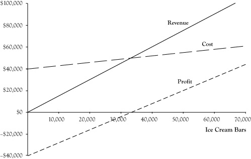
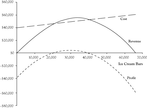
Table 2.1 "Revenue, Cost, and Profit for Selected Sales Volumes for Ice Cream Bar Venture" provides actual values for revenue, cost, and profit for selected values of the volume quantity Q. Figure 2.1 "Graphs of Revenue, Cost, and Profit Functions for Ice Cream Bar Business at Price of $1.50", provides graphs of the revenue, cost, and profit functions.
The average costThe total cost divided by the quantity produced; AC = C/Q. is another interesting measure to track. This is calculated by dividing the total cost by the quantity. The relationship between average cost and quantity is the average cost function. For the ice cream bar venture, the equation for this function would be
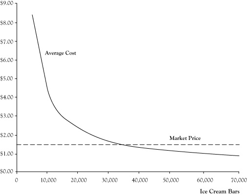
AC = C/Q = ($40,000 + $0.3 Q)/Q = $0.3 + $40,000/Q.Figure 2.2 "Graph of Average Cost Function for Ice Cream Bar Venture" shows a graph of the average cost function. Note that the average cost function starts out very high but drops quickly and levels off.
Table 2.1 Revenue, Cost, and Profit for Selected Sales Volumes for Ice Cream Bar Venture
| Units | Revenue | Cost | Profit |
|---|---|---|---|
| 0 | $0 | $40,000 | –$40,000 |
| 10,000 | $15,000 | $43,000 | –$28,000 |
| 20,000 | $30,000 | $46,000 | –$16,000 |
| 30,000 | $45,000 | $49,000 | –$4,000 |
| 40,000 | $60,000 | $52,000 | $8,000 |
| 50,000 | $75,000 | $55,000 | $20,000 |
| 60,000 | $90,000 | $58,000 | $32,000 |
Figure 2.1 Graphs of Revenue, Cost, and Profit Functions for Ice Cream Bar Business at Price of $1.50
Essentially the average cost function is the variable cost per unit of $0.30 plus a portion of the fixed cost allocated across all units. For low volumes, there are few units to spread the fixed cost, so the average cost is very high. However, as the volume gets large, the fixed cost impact on average cost becomes small and is dominated by the variable cost component.
Figure 2.2 Graph of Average Cost Function for Ice Cream Bar Venture
A scan of Figure 2.1 "Graphs of Revenue, Cost, and Profit Functions for Ice Cream Bar Business at Price of $1.50" shows that the ice cream bar venture could result in an economic profit or loss depending on the volume of business. As the sales volume increases, revenue and cost increase and profit becomes progressively less negative, turns positive, and then becomes increasingly positive. There is a zone of lower volume levels where economic costs exceed revenues and a zone on the higher volume levels where revenues exceed economic costs.
One important consideration for our three students is whether they are confident that the sales volume will be high enough to fall in the range of positive economic profits. The volume level that separates the range with economic loss from the range with economic profit is called the breakeven pointThe volume of business that separates economic loss from economic profit; the quantity at which the revenue function and the cost function are equal.. From the graph we can see the breakeven point is slightly less than 35,000 units. If the students can sell above that level, which the prior operator did, it will be worthwhile to proceed with the venture. If they are doubtful of reaching that level, they should abandon the venture now, even if that means losing their nonrefundable deposit.
There are a number of ways to determine a precise value for the breakeven level algebraically. One is to solve for the value of Q that makes the economic profit function equal to zero:
0 = $1.2 Q − $40,000 or Q = $40,000/$1.2 = 33,334 units.An equivalent approach is to find the value of Q where the revenue function and cost function have identical values.
Another way to assess the breakeven point is to find how large the volume must be before the average cost drops to the price level. In this case, we need to find the value of Q where AC is equal to $1.50. This occurs at the breakeven level calculated earlier.
A fourth approach to solving for the breakeven level is to consider how profit changes as the volume level increases. Each additional item sold incurs a variable cost per unit of $0.30 and is sold for a price of $1.50. The difference, called the unit contribution marginThe difference between the price per unit and the variable cost per unit; price per unit - variable cost per unit., would be $1.20. For each additional unit of volume, the profit increases by $1.20. In order to make an overall economic profit, the business would need to accrue a sufficient number of unit contribution margins to cover the economic fixed cost of $40,000. So the breakeven level would be
Q = fixed cost/(price per unit − variable cost per unit) = $40,000/($1.50 − $0.30) = 33,333.3 or 33,334 units.Once the operating volume crosses the breakeven threshold, each additional unit contribution margin results in additional profit.
We get an interesting insight into the nature of a business by comparing the unit contribution margin with the price. In the case of the ice cream business, the unit contribution margin is 80% of the price. When the price and unit contribution margins are close, most of the revenue generated from additional sales turns into profit once you get above the breakeven level. However, if you fall below the breakeven level, the loss will grow equally dramatically as the volume level drops. Businesses like software providers, which tend have mostly fixed costs, see a close correlation between revenue and profit. Businesses of this type tend to be high risk and high reward.
On the other hand, businesses that have predominantly variable costs, such as a retail grocery outlet, tend to have relatively modest changes in profit relative to changes in revenue. If business level falls off, they can scale down their variable costs and profit will not decline so much. At the same time, large increases in volume levels beyond the breakeven level can achieve only modest profit gains because most of the additional revenue is offset by additional variable costs.
In the preceding analyses of the ice cream venture, we assumed ice cream bars would be priced at $1.50 per unit based on the price that was charged in the previous summer. The students can change the price and should evaluate whether there is a better price for them to charge. However, if the price is lowered, the breakeven level will increase and if the price is raised, the breakeven level will drop, but then so may the customer demand.
To examine the impact of price and determine a best price, we need to estimate the relationship between the price charged and the maximum unit quantity that could be sold. This relationship is called a demand curveThe relationship between the price charged and the maximum unit quantity that can be sold.. Demand curves generally follow a pattern called the law of demandIncreases in price result in decreases in the maximum quantity that can be sold., whereby increases in price result in decreases in the maximum quantity that can be sold.
We will consider a simple demand curve for the ice cream venture. We will assume that since the operator of the business last year sold 36,000 units at a price of $1.50 that we could sell up to 36,000 units at the same price this coming summer. Next, suppose the students had asked the prior operator how many ice cream bars he believes he would have sold at a price of $2.00 and the prior operator responds that he probably would have sold 10,000 fewer ice cream bars. In other words, he estimates his sales would have been 26,000 at a price of $2.00 per ice cream bar.
To develop a demand curve from the prior operator’s estimates, the students assume that the relationship between price and quantity is linear, meaning that the change in quantity will be proportional to the change in price. Graphically, you can infer this relationship by plotting the two price-quantity pairs on a graph and connecting them with a straight line. Using intermediate algebra, you can derive an equation for the linear demand curve
P = 3.3 − 0.00005 Q,where P is price in dollars and Q is the maximum number of ice cream bars that will sell at this price. Figure 2.3 "Linear Demand Curve for Ice Cream Bar Venture" presents a graph of the demand curve.
Figure 2.3 Linear Demand Curve for Ice Cream Bar Venture
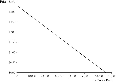
It may seem awkward to express the demand curve in a manner that you use the quantity Q to solve for the price P. After all, in a fixed price market, the seller decides a price and the buyers respond with the volume of demand. Mathematically, the relationship for ice cream bars could be written
Q = 66,000 − 20,000 P.However, in economics, the common practice is to describe the demand curve as the highest price that could be charged and still sell a quantity Q.
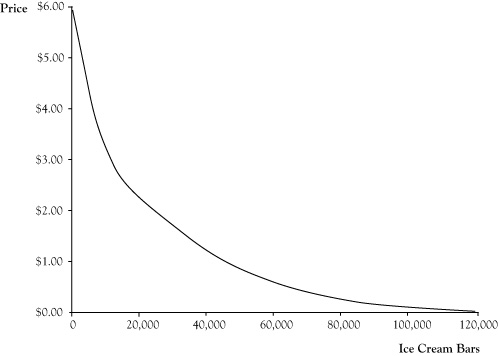
The linear demand curve in Figure 2.3 "Linear Demand Curve for Ice Cream Bar Venture" probably stretches credibility as you move to points where either the price is zero or demand is zero. In actuality, demand curves are usually curved such that demand will get very high as the price approaches zero and small amounts would still sell at very high prices, similar to the pattern in Figure 2.4 "Common Pattern for Demand Curves". However, linear demand curves can be reasonably good estimates of behavior if they are used within limited zone of possible prices.
Figure 2.4 Common Pattern for Demand Curves
We can use the stated relationship in the demand curve to examine the impact of price changes on the revenue and profit functions. (The cost function is unaffected by the demand curve.) Again, with a single type of product or service, revenue is equal to price times quantity. By using the expression for price in terms of quantity rather than a fixed price, we can find the resulting revenue function
R = P Q = (3.3 − 0.00005 Q) Q = 3.3 Q − 0.00005 Q2.By subtracting the expression for the cost function from the revenue function, we get the revised profit function
π = (3.3 Q − 0.00005 Q2) − (40,000 + $0.3 Q) = –0.00005 Q2 + 3 Q − 40,000.Graphs for the revised revenue, cost, and profit functions appear in Figure 2.5 "Graphs of Revenue, Cost, and Profit Functions for Ice Cream Bar Venture for Linear Demand Curve". Note that the revenue and profit functions are curved since they are quadratic functions. From the graph of the profit function, it can be seen that it is possible to earn an economic profit with a quantity as low as 20,000 units; however, the price would need to be increased according to the demand curve for this profit to materialize. Additionally, it appears a higher profit is possible than at the previously planned operation of 36,000 units at a price of $1.50. The highest profitability appears to be at a volume of about 30,000 units. The presumed price at this volume based on the demand curve would be around $1.80.
Figure 2.5 Graphs of Revenue, Cost, and Profit Functions for Ice Cream Bar Venture for Linear Demand Curve
Economists analyze relationships like revenue functions from the perspective of how the function changes in response to a small change in the quantity. These marginal measurementsThe change in a function in response to a small change in quantity; used to determine the optimal level of planned production. not only provide a numerical value to the responsiveness of the function to changes in the quantity but also can indicate whether the business would benefit from increasing or decreasing the planned production volume and in some cases can even help determine the optimal level of planned production.
The marginal revenueThe change in revenue in response to a unit increase in production quantity. measures the change in revenue in response to a unit increase in production level or quantity. The marginal costThe change in cost corresponding to a unit increase in production quantity. measures the change in cost corresponding to a unit increase in the production level. The marginal profitThe change in profit resulting from a unit increase in the quantity sold. measures the change in profit resulting from a unit increase in the quantity. Marginal measures for economic functions are related to the operating volume and may change if assessed at a different operating volume level.
There are multiple computational techniques for actually calculating these marginal measures. If the relationships have been expressed in the form of algebraic equations, one approach is to evaluate the function at the quantity level of interest, evaluate the function if the quantity level is increased by one, and determine the change from the first value to the second.
Suppose we want to evaluate the marginal revenue for the revenue function derived in the previous section at last summer’s operating level of 36,000 ice cream bars. For a value of Q = 36,000, the revenue function returns a value of $54,000. For a value of Q = 36,001, the revenue function returns a value of $53,999.70. So, with this approach, the marginal revenue would be $53,999.70 − $54,000, or –$0.30. What does this tell us? First, it tells us that for a modest increase in production volume, if we adjust the price downward to compensate for the increase in quantity, the net change in revenue is a decrease of $0.30 for each additional unit of planned production.
Marginal measures often can be used to assess the change if quantity is decreased by changing sign on the marginal measure. Thus, if the marginal revenue is –$0.30 at Q = 36,000, we can estimate that for modest decreases in planned quantity level (and adjustment of the price upward based on the demand function), revenue will rise $0.30 per unit of decrease in Q.
At first glance, the fact that a higher production volume can result in lower revenue seems counterintuitive, if not flawed. After all, if you sell more and are still getting a positive price, how can more volume result in less revenue? What is happening in this illustrated instance is that the price drop, as a percentage of the price, exceeds the increase in quantity as a percentage of quantity. A glance back at Figure 2.5 "Graphs of Revenue, Cost, and Profit Functions for Ice Cream Bar Venture for Linear Demand Curve" confirms that Q = 36,000 is in the portion of the revenue function where the revenue function declines as quantity gets larger.
If you follow the same computational approach to calculate the marginal cost and marginal profit when Q = 36,000, you would find that the marginal cost is $0.30 and the marginal profit is –$0.60. Note that marginal profit is equal to marginal revenue minus marginal cost, which will always be the case.
The marginal cost of $0.30 is the same as the variable cost of acquiring and stocking an ice cream bar. This is not just a coincidence. If you have a cost function that takes the form of a linear equation, marginal cost will always equal the variable cost per unit.
The fact that marginal profit is negative at Q = 36,000 indicates we can expect to find a more profitable value by decreasing the quantity and increasing the price, but not by increasing the quantity and decreasing the price. The marginal profit value does not provide enough information to tell us how much to lower the planned quantity, but like a compass, it points us in the right direction.
Since marginal measures are the rate of change in the function value corresponding to a modest change in Q, differential calculus provides another computational technique for deriving marginal measures. Differential calculus finds instantaneous rates of change, so the values computed are based on infinitesimal changes in Q rather than whole units of Q and thus can yield slightly different values. However, a great strength of using differential calculus is that whenever you have an economic function in the form of an algebraic equation, you can use differential calculus to derive an entire function that can be used to calculate the marginal value at any value of Q.
How to apply differential calculus is beyond the scope of this text; however, here are the functions that can be derived from the revenue, cost, and profit functions of the previous section (i.e., those that assume a variable price related to quantity):
marginal revenue at a volume Q = $3.3 − $0.0001 Q, marginal cost at a volume Q = $ 0.3, marginal profit at a volume Q = $3 − $0.0001 Q.Substituting Q = 36,000 into these equations will produce the same values we found earlier. However, these marginal functions are capable of more.
Since the marginal change in the function is the rate of change in the function at a particular point, you can visualize this by looking at the graphs of the functions and drawing a tangent line on the graph at the quantity level of interest. A tangent line is a straight line that goes through the point on the graph, but does not cross the graph as it goes through the point. The slope of the tangent line is the marginal value of the function at that point. When the slope is upward (the tangent line rises as it goes to the right), the marginal measure will be positive. When the slope is downward, the marginal measure will be negative. If the line has a steep slope, the magnitude of the marginal measure will be large. When the line is fairly flat, the magnitude will be small.
Suppose we want to find where the profit function is at its highest value. If you look at that point (in the vicinity of Q = 30,000) on Figure 2.5 "Graphs of Revenue, Cost, and Profit Functions for Ice Cream Bar Venture for Linear Demand Curve", you see it is like being on the top of a hill. If you draw the tangent line, it will not be sloped upward or downward; it will be a flat line with a zero slope. This means the marginal profit at the quantity with the highest profit has a value of zero. So if you set the marginal profit function equal to zero and solve for Q you find
0 = $3.00 − $0.0001 Q implies Q = $3.00/$0.0001 = 30,000.This confirms our visual location of the optimum level and provides a precise value.
This example illustrates a general economic principle: Unless there is a constraint preventing a change to a more profitable production level, the most profitable production levelThe quantity where marginal profit equals zero; in the absence of production level constraints, the quantity where marginal revenue is equal to marginal cost. will be at a level where marginal profit equals zero. Equivalently, in the absence of production level constraints, the most profitable production level is where marginal revenue is equal to marginal cost. If marginal revenue is greater than marginal cost at some production level and the level can be increased, profit will increase by doing so. If marginal cost is greater than marginal revenue and the production level can be decreased, again the profit can be increased.
Our students will look at this analysis and decide not only to go forward with the ice cream business on the beach but to charge $1.80, since that is the price on the demand curve corresponding to a sales volume of 30,000 ice cream bars. Their expected revenue will be $54,000, which coincidently is the same as in the original plan, but the economic costs will be only $49,000, which is lower than in the original analysis, and their economic profit will be slightly higher, at $5000.
At first glance, a $5000 profit does not seem like much. However, bear in mind that we already assigned an opportunity cost to the students’ time based on the income foregone by not accepting the corporate internships. So the students can expect to complete the summer with $10,000 each to compensate for the lost internship income and still have an additional $5000 to split between them.
You may recall earlier in this chapter that, before deciding to disregard the $6000 nonrefundable down payment (to hold the option to operate the ice cream business) as a relevant economic cost, the total cost of operating the business under a plan to sell 36,000 ice cream bars at a price of $1.50 per item would have exceeded the expected revenue. Even after further analysis indicated that the students could improve profit by planning to sell 30,000 ice cream bars at a price of $1.80 each, if the $6000 deposit had not been a sunk cost, there would have been no planned production level and associated price on the demand curve that would have resulted in positive economic profit. So the students would have determined the ice cream venture to be not quite viable if they had known prior to making the deposit that they could instead each have a summer corporate internship. However, having committed the $6000 deposit already, they will gain going forward by proceeding to run the ice cream bar business.
A similar situation can occur in ongoing business concerns. A struggling business may appear to generate insufficient revenue to cover costs yet continue to operate, at least for a while. Such a practice may be rational when a sizeable portion of the fixed costs in the near term are effectively sunk, and the revenue generated is enough to offset the remaining fixed costs and variable costs that are still not firmly committed.
Earlier in the chapter, we cited one condition for reaching a breakeven production level where revenue would equal or exceed costs as the point where average cost per unit is equal to the price. However, if some of the costs are already sunk, these should be disregarded in determining the relevant average cost. In a circumstance where a business regards all fixed costs as effectively sunk for the next production period, this condition becomes a statement of a principle known as the shutdown ruleWhen all fixed costs are regarded as sunk for the next production period, a firm should continue to operate only as long as the selling price per unit is at least as large as the average variable cost per unit.: If the selling price per unit is at least as large as the average variable cost per unit, the firm should continue to operate for at least a while; otherwise, the firm would be better to shut down operations immediately.
Two observations about the shutdown rule are in order: In a circumstance where a firm’s revenue is sufficient to meet variable costs but not total costs (including the sunk costs), although the firm may operate for a period of time because the additional revenue generated will cover the additional costs, eventually the fixed costs will need to be refreshed and those will be relevant economic costs prior to commitment to continue operating beyond the near term. If a business does not see circumstances changing whereby revenue will be getting better or costs will be going down, although it may be a net gain to operate for some additional time, such a firm should eventually decide to close down its business.
Sometimes, it is appropriate to shut down a business for a period of time, but not to close the business permanently. This may happen if temporary unfavorable circumstances mean even uncommitted costs cannot be covered by revenue in the near term, but the business expects favorable conditions to resume later. An example of this would be the owner of an oil drilling operation. If crude oil prices drop very low, the operator may be unable to cover variable costs and it would be best to shut down until petroleum prices climb back and operations will be profitable again. In other cases, the opportunity cost of resources may be temporarily high, so the economic profit is negative even if the accounting profit would be positive. An example would be a farmer selling his water rights for the upcoming season because he is offered more for the water rights than he could net using the water and farming.
In the example used in this chapter, we assumed the students’ goal in how to operate the ice cream business was to maximize their profit—more specifically, to maximize their economic profit. Is this an appropriate overall objective for most businesses?
Generally speaking, the answer is yes. If a business is not able to generate enough revenue to at least cover their economic costs, the business is losing in the net. In addition to the business owners having to cover the loss out of their wealth (or out of society’s largesse for a bankruptcy), there is an inefficiency from a societal perspective in that the resources used by the business could be more productive elsewhere.
The ice cream business analyzed here was simple in many respects, including that it was intended to operate for only a short period of time. Most businesses are intended to operate for long periods of time. Some businesses, especially newly formed businesses, will intentionally operate businesses at a loss or operate at volumes higher than would generate the maximum profit in the next production period. This decision is rational if the business expects to realize larger profits in future periods in exchange for enduring a loss in the near future. There are quantitative techniques, such as discounting,Many accounting and economics texts discuss the concept of discounting of profits over time. One good discussion can be found in an appendix in Hirschey and Pappas (1996). that allow a business decision maker to make these trade-offs between profit now and profit later. These techniques will not be covered in this text.
Economists refer to a measure called the value of the firmThe collective worth of all economic profits into the future and the amount the owners would expect to receive if they sold the business; for a corporation, the equity on a company's balance sheet., which is the collective value of all economic profits into the future and approximately the amount the owners should expect to receive if they sold the business to a different set of owners. For a corporation, in theory this would roughly equate to the value of the equity on a company’s balance sheet, although due to several factors like sunk costs, is probably not really that value. Economists would say that a business should make decisions that maximize the value of the firm, meaning the best decisions will result in larger economic profits either now or later.
One response to the principle that the overall goal of a firm is to maximize its value is that, although that goal may be best for those who own the business, it is not the optimal objective for the overall society in which the business operates. One specific objection is that those who work for the business may not be the same as those who own the business and maximizing the value for the owners can mean exploiting the nonowner employees. The common response to this objection is that it will be in the owners’ best interest in the long run (several periods of operation) to treat their employees fairly. Businesses that exploit their employees will lose their good employees and fail to motivate those employees who remain. The collective result will be lower profits and a lower value of the firm.
A second objection to the appropriateness of operating a business to maximize the value for the owners is that this invites businesses to exploit their customers, suppliers, and the society in which they operate to make more money. Firms may be able to take advantage of outside parties for a while, but eventually the customers and suppliers will wise up and stop interacting with the business. With a high level of distrust, there will be a decline in profits in future periods that will more than offset any immediate gain. If a business tries to exploit the overall society by ruining the environment or causing an increase in costs to the public, the business can expect governmental authorities to take actions to punish the firm or limit its operations, again resulting in a net loss over time. So maximizing the value of the firm for the owners does not imply more profit for the owners at the expense of everyone else. Rather, a rational pursuit of maximal value will respect the other stakeholders of a business.
In the case of nonprofit organizations, maximizing the value of the organization will be different than with for-profit businesses like our ice cream example. A nonprofit organization may be given a budget that sets an upper limit on its costs and is expected to provide the most value to the people it serves. Since most nonprofit organizations do not charge their “customers” in the same way as for-profit businesses, the determination of value will be different than estimating sales revenue. Techniques such as cost-benefit analysisA classic text in cost-benefit analysis was written by E. J. Mishan (1976). have been developed for this purpose.


