In this chapter we have examined the model of utility-maximizing behavior. Economists assume that consumers make choices consistent with the objective of achieving the maximum total utility possible for a given budget constraint.
Utility is a conceptual measure of satisfaction; it is not actually measurable. The theory of utility maximization allows us to ask how a utility-maximizing consumer would respond to a particular event.
By following the marginal decision rule, consumers will achieve the utility-maximizing condition: Expenditures equal consumers’ budgets, and ratios of marginal utility to price are equal for all pairs of goods and services. Thus, consumption is arranged so that the extra utility per dollar spent is equal for all goods and services. The marginal utility from a particular good or service eventually diminishes as consumers consume more of it during a period of time.
Utility maximization underlies consumer demand. The amount by which the quantity demanded changes in response to a change in price consists of a substitution effect and an income effect. The substitution effect always changes quantity demanded in a manner consistent with the law of demand. The income effect of a price change reinforces the substitution effect in the case of normal goods, but it affects consumption in an opposite direction in the case of inferior goods.
An alternative approach to utility maximization uses indifference curves. This approach does not rely on the concept of marginal utility, and it gives us a graphical representation of the utility-maximizing condition.
The table shows the total utility Joseph derives from eating pizza in the evening while studying.
| Pieces of pizza/evening | Total Utility |
|---|---|
| 0 | 0 |
| 1 | 30 |
| 2 | 48 |
| 3 | 60 |
| 4 | 70 |
| 5 | 78 |
| 6 | 80 |
| 7 | 76 |
The table shows the total utility (TU) that Jeremy receives from consuming different amounts of two goods, X and Y, per month.
| Quantity | TUX | MUX | MUX/PX | TUY | MUY | MUY/PY |
|---|---|---|---|---|---|---|
| 0 | 0 | 0 | ||||
| 1 | 50 | 75 | ||||
| 2 | 88 | 117 | ||||
| 3 | 121 | 153 | ||||
| 4 | 150 | 181 | ||||
| 5 | 175 | 206 | ||||
| 6 | 196 | 225 | ||||
| 7 | 214 | 243 | ||||
| 8 | 229 | 260 | ||||
| 9 | 241 | 276 |
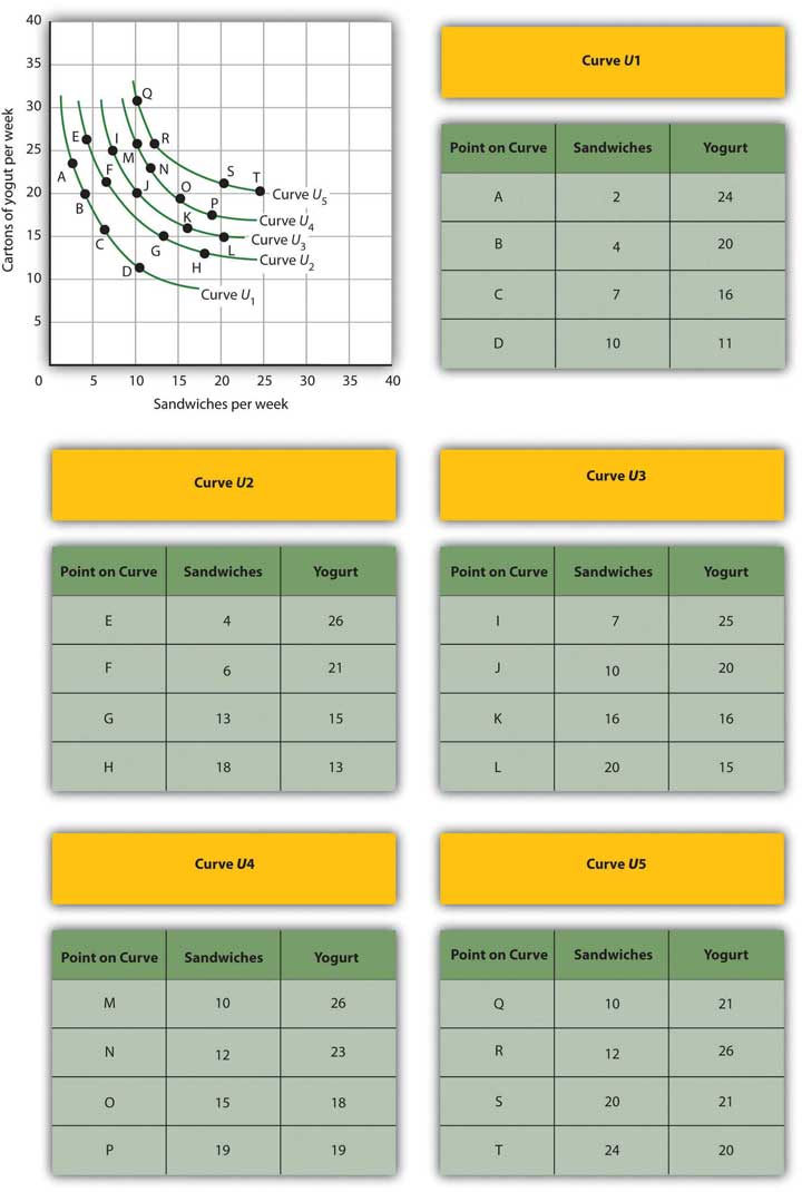
Sid is a commuter-student at his college. During the day, he snacks on cartons of yogurt and the “house special” sandwiches at the Student Center cafeteria. A carton of yogurt costs $1.20; the Student Center often offers specials on the sandwiches, so their price varies a great deal. Sid has a budget of $36 per week for food at the Center. Five of Sid’s indifference curves are given by the schedule below; the points listed in the tables correspond to the points shown in the graph.

Consider a consumer who each week purchases two goods, X and Y. The following table shows three different combinations of the two goods that lie on three of her indifference curves—A, B, and C.
| Indifference Curve | Quantities of goods X and Y, respectively | Quantitities of goods X and Y, respectively | Quantities of goods X and Y, respectively |
|---|---|---|---|
| A | 1 unit of X and 4 of Y | 2 units of X and 2 of Y | 3 units of X and 1 of Y |
| B | 1 unit of X and 7 of Y | 3 units of X and 2 of Y | 5 units of X and 1 of Y |
| C | 2 units of X and 5 of Y | 4 units of X and 3 of Y | 7 units of X and 2 of Y |