So far we have discussed how you choose to spend your money. There is another decision you make every day: how to spend your time. You have 24 hours each day in which to do all the different things you want to do: work, sleep, eat, study, watch television, surf the Internet, go to the movies, and so on. Time, like money, is scarce. Given that you have only 24 hours to allocate in every day, how do you decide which activities to spend your time on? This problem is very similar to the allocation of your budget, with one key difference: you cannot save or borrow time in the way that you can save or borrow money. There are exactly 24 hours in each day—no more, no less.
We begin with the most fundamental time allocation problem for all students: choosing between studying and sleeping. As before, we keep things simple by thinking about only two possible uses of your time. You are given 24 hours in the day to study and sleep. How should you allocate your time?
As with the allocation of your income, there are two aspects of this problem. First, there is a budget constraint—only now it is your time that is scarce, not money. Second, you have your own preferences about sleep and study time. Your ability to meet your desires is constrained by the scarcity of your time: you must trade off one activity for another.
The time budget constraintThe restriction that the sum of the time you spend on all your different activities must be exactly 24 hours each day. is the restriction that there are only 24 hours in the day. It is shown in Figure 4.14 "The Time Budget Constraint" and is the counterpart to the budget line in our earlier discussion. Any point in this figure represents a combination of sleep and study time. The sum of sleep and study time must equal 24 hours (remember we are supposing that these are the only ways you spend your time). Thus your allocation of your time must lie somewhere on this line.
Figure 4.14 The Time Budget Constraint
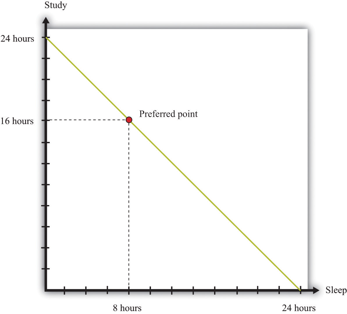
The time allocation line shows your options for dividing your time between study and sleep.
Figure 4.14 "The Time Budget Constraint" also shows one possible choice that you might make: allocating 8 hours to sleep and 16 hours to studying. The choice of this point reflects your desires for sleep and study. As with the spending decision, we pass no judgment, as economists, on the actual decision you make. We suppose you typically make the choice that makes you the happiest.
At your preferred point, your choice to sleep for 8 hours means that your study time must equal 16 hours; equivalently, your choice to study for 16 hours means that you must sleep for 8 hours. Any increase in one activity must be met by a reduction in time for the other. The opportunity cost of each hour of sleep is an hour of study time, and the opportunity cost of each hour of study time is an hour of sleep. If you choose this point, you reveal that you are willing to “pay” (that is, give up) 8 hours of study time to obtain 8 hours of sleep, and you are willing to pay 16 hours of sleep to obtain 16 hours of study time.
As with consumption choices, it is often enough to look at small changes to evaluate whether or not you are making a good decision. The opportunity cost of a little more sleep is a little less study time. If you are making a good decision about the allocation of your time, then the extra sleep is not worth the extra study time. Suppose you are contemplating a particular point on the time budget line, and you want to know if it is a good choice. If a very small movement away from your chosen point will not make you happier, then—in most circumstances—neither will a big movement. By a very small movement, we mean sleeping a little less and studying a little more or studying a little less and sleeping a little more. If you are making a good decision, then your willingness to substitute sleep for study time is exactly the same as that allowed by the time constraint.
Sleeping and studying are uses of your time that are directly for your own benefit. Most people—perhaps including yourself—also spend time working for money. So let us now look at the choice between spending time working and enjoying leisure. Our goal is to determine how much labor you will choose to supply to the market—which is equivalently a choice about how much leisure time to enjoy, because choosing the number of working hours is the same as choosing the number of leisure hours. Your choice between the two is based on the trade-off between enjoying leisure and working to earn money that allows the purchase of goods.
Once again—to make it easy to draw diagrams—we suppose that these are the only uses of your time. Part (a) of Figure 4.15 "Choosing between Work and Leisure" presents the allocation of time between work and leisure. As with the sleep-study choice, there is a time budget constraint, and you have preferences between these two ways to allocate time. Your best choice satisfies the same property as before: you allocate time such that no other division of your time makes you happier.
What makes this different from the sleep-study choice is the valuation of your time. We can think of sleep as a good thing in that you generally prefer more to less. Likewise, we can think of study as a good thing in that—even if you don’t always enjoy it—you perceive a gain to spending time studying. So Figure 4.14 "The Time Budget Constraint" is like our earlier diagrams with downloads and chocolate bars: it has a good thing on each axis. Now, people presumably prefer more leisure to less: leisure is a “good,” like chocolate bars, blue jeans, or cans of soda. But we have drawn part of (a) Figure 4.15 "Choosing between Work and Leisure" as if work is also a good thing. Most people, however, see work time as a “bad” rather than as a “good.” Even people who like their work would almost always prefer to work a little less and have a little more leisure time.
Figure 4.15 Choosing between Work and Leisure
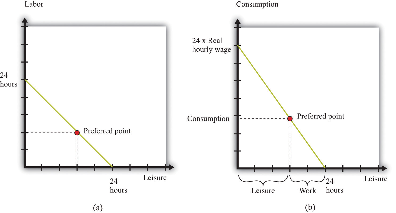
(a) The time budget line shows your options for dividing your time between labor and leisure. However, we generally think of labor as a “bad” rather than as a “good.” (b) Now the choice is between consumption and leisure. For each hour of your time, you earn the nominal hourly wage. If you divide this by the price level, you get the real wage. The real wage tells you how many goods and services you can enjoy for one hour of work.
The gain from working, of course, is that you earn income, allowing you to purchase goods and services. Each extra hour of your work allows you to buy more goods and services. Conversely, if you want more leisure time, you must give up some goods and services. Thus the choice between labor and leisure is linked to the choice about how many chocolate bars and other goods you buy. The income we take as given in describing your budget set typically comes from your decision to supply labor time. (Of course, you may have other sources of income as well, such as loans or grants.)
Part (b) of Figure 4.15 "Choosing between Work and Leisure" takes the labor-leisure choice and converts it into a choice between leisure and consumption. Here, consumption refers to all the goods and services you consume. We lump together all the products you consume, just as we lump together all your different forms of leisure (sleep, study, watching television, and so on). As before, time is measured on the horizontal axis: there are 24 hours to the day, which must be split between leisure time and labor time. On the vertical axis, we measure consumption.
To get the budget constraint for this picture, we begin with the time budget constraint:
leisure hours + labor hours = 24.The value of an hour of time in dollars is given by the wages at which you can sell your time. Multiplying the time budget constraint by the wage gives us a budget constraint in dollars:
(leisure hours × wage) + wage income = 24 × wage.Wage income is equal to the number of hours worked times the hourly wage. Because wage income is used to buy goods, we can replace it by total spending on consumption, which is the price level times the quantity of consumption goods purchased:
(leisure hours × wage) + (price level × consumption) = 24 × wage.This is the budget constraint faced by an individual choosing between leisure and consumption. Think of it as follows: The individual first sells all her labor at the going wage, yielding the income on the right-hand side. With this income, she then “buys” back leisure and also buys consumption goods. The price of an hour of leisure represents the wage rate, and the price of a unit of consumption goods represents the price level.
Toolkit: Section 31.3 "The Labor Market"
The real wage is the relative price of labor in terms of consumption goods:
Dividing the time budget constraint by the price level, we get the budget in line in part (b) of Figure 4.15 "Choosing between Work and Leisure".
leisure hours × real wage + consumption = 24 × real wage.As you move along the budget line, you trade hours of leisure for consumption goods. The slope of the budget line is the negative of the real wageThe nominal wage (the wage in dollars) divided by the price level.. If you give up an hour of leisure, you obtain extra consumption equal to the real wage. Put differently, the opportunity cost of an hour of leisure is the amount of consumption you give up by not working. Once we have worked out how much leisure you consume, we have equivalently worked out how much labor you supply:
labor hours = 24 − leisure hours.Part (a) of Figure 4.16 "The Effect of a Real Wage Increase on the Quantity of Labor Supplied" shows what happens when the real wage changes. When the real wage increases, the vertical intercept of the budget line is higher because the vertical intercept tells us how much consumption an individual could obtain if she worked for all 24 hours in the day. The horizontal intercept does not change as the real wage changes: if an individual does not work, then the level of consumption is zero regardless of wages. It follows that the budget line is steeper as the real wage increases. If an individual gives up an hour of leisure time, he or she gets more additional consumption when the real wage is higher. The opportunity cost of leisure in terms of forgone consumption is higher.
Figure 4.16 The Effect of a Real Wage Increase on the Quantity of Labor Supplied
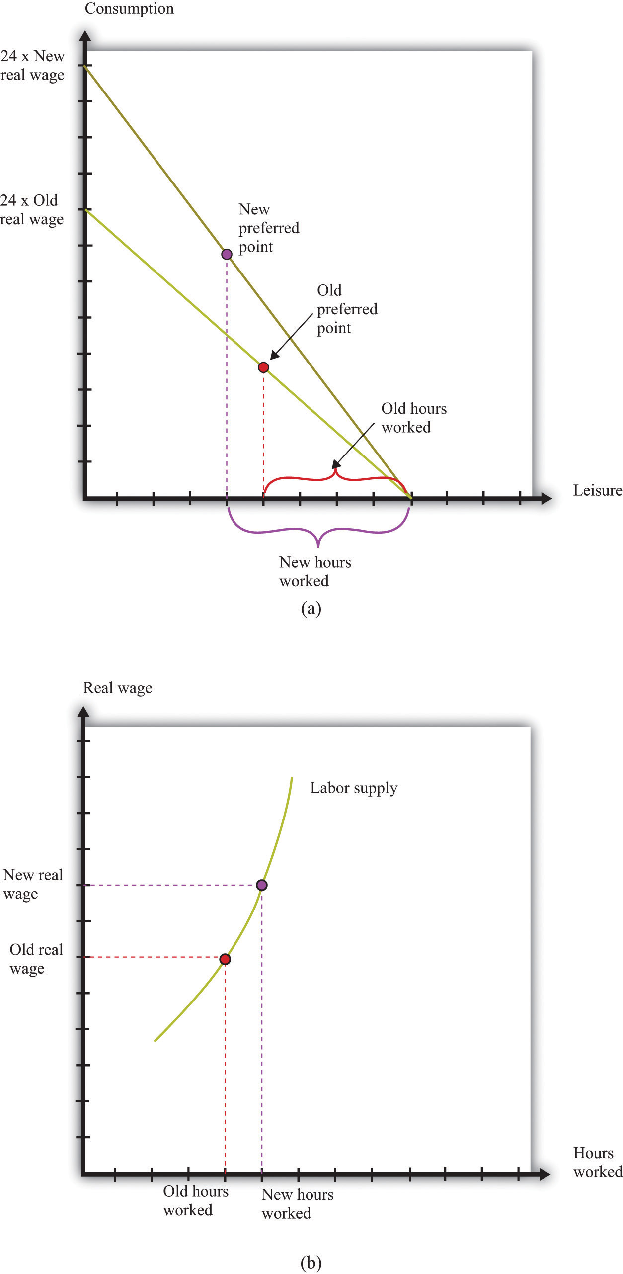
(a) An increase in the real wage causes the budget line to rotate. Income and substitution effects are both at work: the income effect encourages more leisure (less work), while the substitution effect encourages more work. The substitution effect generally dominates, so higher real wages lead to more work. This means that the labor supply curve slopes upward, as shown in (b).
Part (b) of Figure 4.16 "The Effect of a Real Wage Increase on the Quantity of Labor Supplied" shows the individual labor supply curveA curve that indicates how many hours of labor an individual supplies at different values of the real wage. that emerges from the labor-leisure choice.
Toolkit: Section 31.3 "The Labor Market"
The individual labor supply curve shows the number of hours that an individual chooses to work at each value of the real wage.
In fact, there are conflicting incentives at work here. As the real wage increases, the opportunity cost of leisure is higher, so you are tempted to work more. But at a higher real wage, you can enjoy the same amount of consumption with fewer hours of work, so this tempts you to work less. This is another example of substitution and income effects. The substitution effect says that when something gets more expensive, we buy less of it. When the real wage increases, leisure is more expensive. The income effect says that as the real wage increases, you can buy more of the things you like, including leisure. We know from our study of demand that, for normal goods, the income and substitution effects act in the same direction. In the case of supply, however, income and substitution effects point in different directions. Consistent with this, most economic studies find that, though the labor supply curve slopes upward, hours worked are not very responsive to changes in the real wage.
Some jobs do not give you any control over the number of hours that you must work. Labor supply then becomes a “unit supply” decision, analogous to the unit demand decisions we considered previously. Should you take a job at all and, if so, what job? To the extent that you can choose among different jobs that offer different hours of work, your decision about whether or not to work will still reflect a trade-off between leisure and consumption.
We have discussed almost everything in this chapter in terms of an individual’s decision making. However, economists often think in terms of households rather than individuals. In part this is because—as we saw with the budget studies—much more economic data are collected for households than for individuals. Also, many of the decisions we have discussed are really made by a household as a whole, rather than by the individual members of that household.
For example, many households have two working adults. Their decisions about how much to work will usually be made jointly on the basis of the real wages they both face. To see some implications of this, consider a two-person household in which both are working. Now suppose that the real wage increases for one person in the household. One person will probably respond by increasing the number of hours worked. However, the other person may choose to work less. Imagine, for example, that there are household chores that either could do. By working less, one person can do more of these chores and thus compensate the other person for the extra hours worked.This is an application of an important economic idea called comparative advantage, which we discuss in more detail in Chapter 6 "eBay and craigslist". Most of the time, though, we do not need to worry about the distinction between the individual and the household, and we often use the terms interchangeably.
Table 4.6 "Allocation of Hours in a Day" shows the allocation of time to certain activities for individuals in three countries: the United States, the United Kingdom, and Mexico. It shows the time allocated on average per day for each of four activities: work, study, personal care, and leisure.
Table 4.6 Allocation of Hours in a Day
| Country | Age | Work | Study | Personal Care | Leisure |
|---|---|---|---|---|---|
| United States | 15–24 | 2.65 | 2.2 | 9.95 | 5.46 |
| United Kingdom | 16–24 | 3.00 | 1.39 | 9.96 | 5.13 |
| Mexico | 20–29 | 4.49 | 0.72 | 10.37 | 3.1 |
For the United States and the United Kingdom, the average number of hours worked is between 2.65 and 3.00. This is an average: some people in this age group may work a full-time job, while others may be students who are not working for pay at all. The sample from Mexico differs from the US and UK samples. First, the group is slightly older. Second, Mexico is notably poorer than the United States and the United Kingdom. For these two reasons, individuals sampled in Mexico are more likely to be working and less likely to be studying and enjoying leisure—which is indeed what we see.
So far we have looked at the allocation of your income separately from the allocation of your time. Yet these choices are linked. The allocation of your time influences the income you have to spend on goods and services. So a change in the wages you are paid will affect how you allocate your time and the goods and services you choose to buy.
In a similar fashion, the prices of goods and services you purchase will have an influence on your allocation of time. For example, if the price of a computer you want to buy decreases, you may respond by working a little more to earn extra income to purchase the computer. The reduction in the price of the computer raises your real wage, so you respond by working more.
If the real wage changes, there are changes in both consumption decisions and work choices. Figure 4.16 "The Effect of a Real Wage Increase on the Quantity of Labor Supplied" shows that an increase in the real wage means you can obtain more consumption for a given amount of work time. Further, as in Figure 4.6 "An Increase in Income", the budget set expands as income increases. Because an increase in the real wage will lead to an increase in hours worked (see Figure 4.16 "The Effect of a Real Wage Increase on the Quantity of Labor Supplied"), labor income will increase. So we can interpret the shift in the budget line in Figure 4.6 "An Increase in Income" as coming from this increase in labor income.
When income increases, you will generally consume more of all goods and services. An increase in the real wage leads to an outward shift in your demand curves for chocolate bars, downloads, and all other normal goods. Combining these figures, we can make the following predictions about the effects of an increase in the real wage:
The last item in the list draws on Figure 4.6 "An Increase in Income" but is less direct than the other implications. As the real wage—and thus your income—increases, the set of bundles you can afford is larger. Moreover, every bundle you could afford when you had less income is still affordable now that you have more income. Thus we conclude that you will be happier. After all, you can always purchase the bundle you bought with lower income and still have some extra income to spend.
Suppose the price of a chocolate bar increases. We saw from Figure 4.8 "A Decrease in the Price of a Chocolate Bar" that when this price increases, the budget set shrinks. We also saw from Figure 4.9 "The Demand Curve" that the demand for chocolate bars decreases when the price of a chocolate bar increases. But there are also implications for labor supply. Remember that the real wage is the nominal wage dividing by a price index representing a household’s cost of purchasing a bundle of goods and services. So when the price of a chocolate bar increases, the cost of purchasing the bundle will increase and the real wage will decrease. From Figure 4.16 "The Effect of a Real Wage Increase on the Quantity of Labor Supplied", labor supply will decrease as the real wage decreases. This is a movement along the labor supply curve.


