Figure 9.1 "Walmart Fact Sheet" is a fact sheet from Walmart. The fact sheet tells you—if you didn’t know already—that Walmart is everywhere. It has over 7,000 retail units in the world, with over 3,000 outside the United States. Walmart employs about 1.36 million people in the United States alone, which is about 1 percent of the total number of workers employed in the United States. It seems that Walmart means jobs.
Figure 9.2 Walmart: Growing Jobs?

Source: This image is taken from http://en.wikipedia.org/wiki/Image:Walmartbizarro.png. The image is copyright Dan Piraro 2006.
Despite the fact that Walmart provides so many jobs, the announcement of a new Walmart store is often greeted with trepidation or outright opposition. There are websites and even a film (http://www.walmartmovie.com) dedicated to criticism of Walmart. It is true that the arrival of Walmart in a town will mean the creation of new jobs, including checkout clerks, shelf packers, and many other positions. Yet the arrival of Walmart will also mean that its competitors will lose jobs. The overall effect on jobs is unclear.
The arrival of a Walmart in a town has implications beyond the effects on jobs. Consumers are likely to face a different menu of goods. Walmart will bring some goods that were previously unavailable, while at the same time other goods sold by unsuccessful specialty stores will disappear. The shopping experience will change for consumers because shopping in a Walmart is not like shopping in a series of small stores. Consumers will face different and—for the most part—lower prices: Walmart is able to obtain goods more cheaply from suppliers and also has a very efficient distribution system that decreases costs. As fewer consumers visit the smaller shops, other nearby businesses, such as local restaurants, may suffer a decline in demand. The patterns of life in the town will change in numerous yet subtle ways.
This scenario has played out in many countries with many different stores. In France, there are hypermarkets such as Carrefour that likewise have had major effects on local businesses and sometimes encounter opposition. In England, the same is true of the Asda supermarket chain. In this chapter, we look at the economics that lies behind a firm’s decision to enter new markets (that is, open new stores) and exit from markets (that is, close down and go out of business). Although we begin here with Walmart, we tell a story that is about much more. Over the course of every year, jobs are created when existing firms expand and new firms enter. At the same time, jobs are lost when firms contract their workforces or close down completely.
A job is created when either an existing firm or a new firm hires workers. Jobs are destroyed when a firm fires some of its workers, some workers quit, or a firm exits a market. Figure 9.3 "US Net Job Creation from 2000 to 2009" provides data on net job creation in the United States from 2000 to 2009. By net job creation, we mean the number of new jobs created minus the number of jobs destroyed. For example, if some firms expand their employment by 200 workers and other firms reduce their workforce by 150 workers, we say that 200 jobs are created, 150 are destroyed, and the net job creation is 50.
Figure 9.3 US Net Job Creation from 2000 to 2009
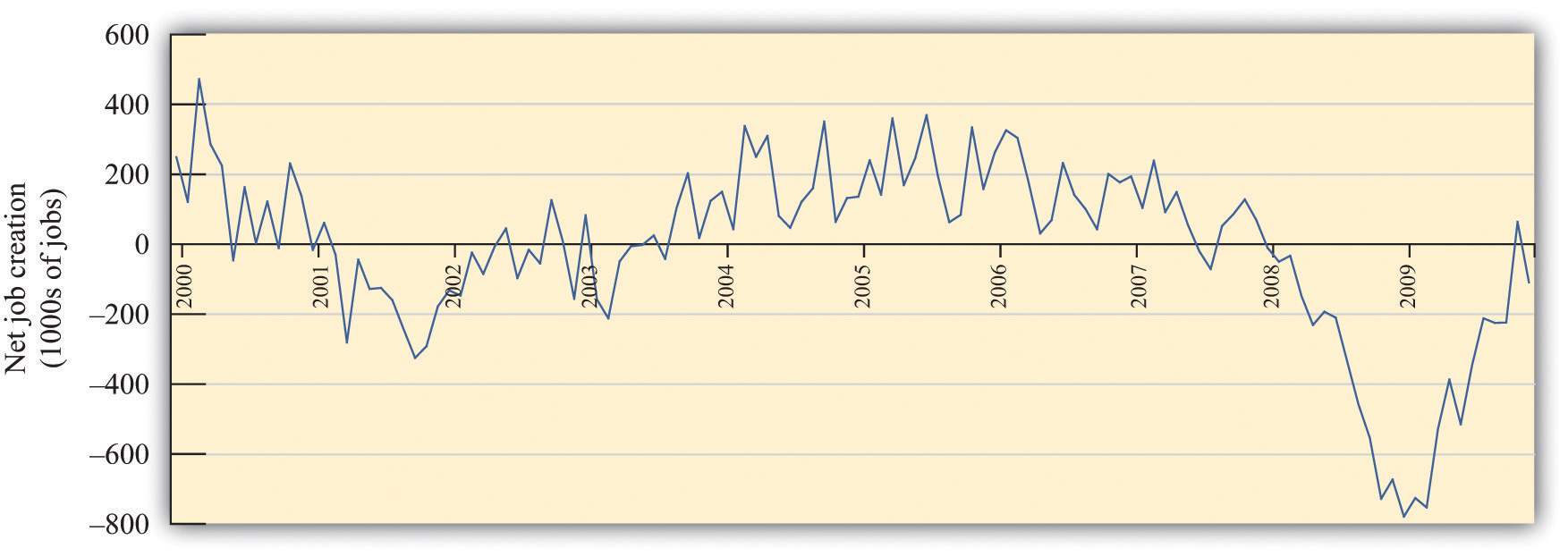
Job creation and destruction take place all the time. Within an industry, and sometimes even within a firm, we see job creation and destruction occurring simultaneously. The Bureau of Labor Statistics now regularly produces quarterly job creation and destruction rates for the US economy.See Bureau of Labor Statistics, Business Employment Dynamics, “Table 3. Private sector gross job gains and losses, as a percent of employment, seasonally adjusted,” accessed March 1, 2011, http://www.bls.gov/web/cewbd/table3_1.txt. For the US private sector over the period 1990–2010, the average quarterly job creation and destruction rates were 7.5 percent and 7.3 percent, respectively. To put it another way, if you looked at 1,000 typical private sector jobs right now, then 75 of them didn’t exist last quarter, and 73 won’t exist next quarter. This implies that about 15 percent of jobs are either destroyed or created in a given quarter. Steven Davis, John Haltiwanger, and Scott Schuh, who were perhaps the first economists to study these processes in detail, call this job reallocation because it reflects the reshuffling of jobs across production locations. Sometimes a car produced at one particular automobile factory is selling well, so new jobs are created there. In the same quarter, another automobile factory may be shut down because the models produced there are not selling. The picture you should take away from these numbers is one of a very fluid labor market. One of our goals in this chapter is to understand how this labor market works.
One way that jobs can be created is by expanding an existing plant or firm. Another way that jobs are created is by the entry of a new plant or firm. The situation is analogous for job destruction. Some jobs are lost when existing plants contract (such as a plant eliminating a shift). Others are lost through the exit of a plant or a firm. The Davis, Haltiwanger, and Schuh data suggest that, each quarter, 11.5 percent of the jobs destroyed come from plants closing. An additional 20 percent of jobs are destroyed when plants undertake large workforce adjustments of more than 50 percent. On the entry side, about 8.4 percent of jobs created in a quarter are due to start-ups. Of course, if these start-ups are successful, then they create more jobs in later years. Ultimately, we want to answer the following question:
What are the economic forces driving job creation and destruction?
The first part of this chapter examines labor demand by firms. We begin by looking at the decision of how many hours to hire. Then we turn to the entry and exit decisions of firms. We find the decision rules that govern these decisions.
After that, we consider a different way of looking at the labor market by examining the process of search and bargaining. We look at how workers who supply labor and firms that demand labor actually interact. Finally, we examine the effects of various government policies on labor market outcomes.
When economists are asked to explain the creation and destruction of jobs in an economy, they will typically begin with a diagram of supply and demand in the labor market. In the labor market, the real wage (on the vertical axis) and the total number of hours worked (on the horizontal axis) are determined by the interaction of labor supply and labor demand. As shown in Figure 9.4 "Labor Market Equilibrium", equilibrium in the labor market occurs at the wage and employment level such that the number of hours supplied and demanded is equal.
Figure 9.4 Labor Market Equilibrium
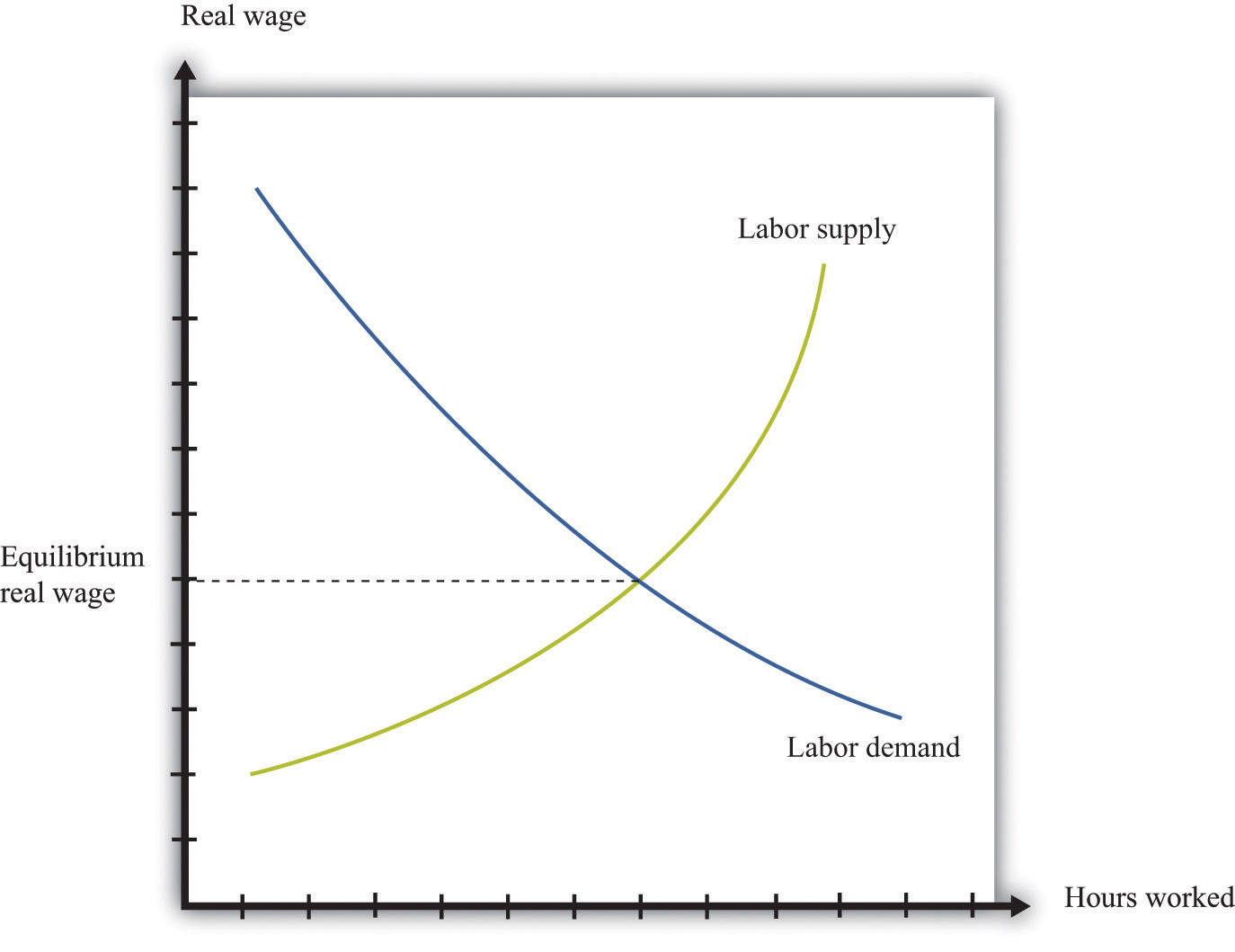
The equilibrium real wage in the labor market is the price where supply equals demand.
Toolkit: Section 31.3 "The Labor Market"
See the toolkit for more discussion on the labor market.
The upward-sloping supply curve tells us that households will want to supply more labor time as wages increase.Labor supply is discussed in Chapter 4 "Everyday Decisions".
Labor demand slopes downward for two analogous reasons:
Thus an increase in wages will induce job destruction, and a decrease in wages will induce job creation.
Firms hire labor to help them produce output. The amount of labor that a firm needs depends on the amount of output that it wants to produce. At the same time, its decision about how much to produce depends on its costs of production, which include the cost of labor. Our task here is to combine these ideas. The decision about how much labor to hire is only one of a large number of choices made by a firm’s managers. Of these, the most fundamental decisions are the following:
A firm’s managers should actually answer these questions in the reverse order:
We follow this logic in our discussion.
Toolkit: Section 31.15 "Pricing with Market Power"
You can review the demand curve facing a firm and the details of pricing with market power in the toolkit.
A firm possesses a means of turning inputs into outputs. For example, Starbucks produces, among other things, grande vanilla low-fat decaf lattes. This drink is an example of a Starbucks output. The list of inputs that Starbucks needs to produce this product is much too long to write out in full but includes the following:
This list doesn’t include any of the “back office” aspects of Starbucks’ operations, such as accounting, payroll, or the logistics of sourcing coffee beans and delivering them to individual stores. Other firms, of course, would have a very different list of inputs. So if we want to talk in abstract terms about the production of a firm, we need a description of production that could apply not only to Starbucks but also to General Motors, IKEA, your local computer repair store, and a manufacturer of paper clips. Therefore, we group inputs into broad categories called factors of productionThe inputs used in a firm’s production process, primarily physical capital, labor hours, raw materials, and technology..
Toolkit: Section 31.17 "Production Function"
Economists group the inputs of any firm into a small number of general categories: raw materials, capital, and labor. We call these inputs a firm’s factors of production.
You can think of raw materials as the things that are transformed in the production process. In our Starbucks example, these include milk, coffee beans, and electricity. Labor refers to the time of the employees who work at a firm, so the time put in by a Starbucks’ barista counts as labor. Capital refers to goods that are used to help with production but are not used up in the process. The espresso machine is one of Starbucks’ capital goods; others are the tables and chairs in the café.
Starbucks’ technologyA means of producing output from inputs.—which we also think of as a factor of production—is the knowledge that allows it to take all these inputs and turn them into an output—the final product that people actually want to buy. It is this knowledge that ultimately lies behind Starbucks’ existence as a firm. Included in the technology are the managerial skills that allow Starbucks to operate effectively.
Figure 9.5 The Technology of a Firm
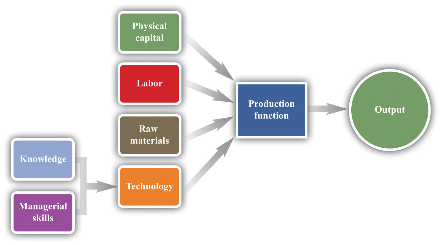
The production function combines a firm’s physical capital stock, labor, raw materials, and technology to produce output. Technology is the knowledge (the blueprints) that a firm possesses, together with managerial skills.
We represent the production process of a firm schematically in Figure 9.5 "The Technology of a Firm". Our description is quite general and can apply to nearly any kind of firm—for example, a lawyer’s office, Walmart, a university, and a child’s lemonade stand. Most people find it easiest to visualize a production function in terms of physical manufacturing, such as a production line for automobiles. Think of a firm’s capital as factory buildings and machinery; its labor as the workers on the production line; and its raw materials as the steel, plastic, and glass that it purchases.
We summarize the technological possibilities of a firm using a production functionA description of how much output a firm can produce as it varies its inputs., which is a description of how much output a firm can produce as it varies its inputs. Even though a typical firm’s production function contains many different inputs, we can understand most of the key features of the production function using an example where labor is the only factor of production. Although there are few goods or services that literally require no inputs other than labor, there are many services that are highly labor intensive, such as babysitting, housecleaning, and personal training at a gym.
To be concrete, think about housecleaning and suppose it has the following production function:
output = productivity × hours of labor input,where we think of productivity as just some number. If output measures clean houses, and if it takes 5 hours of labor to produce one clean house, then productivity is 0.2, and the production function is
output = 0.2 × hours of labor input.The production function tells us the level of output of a firm for given levels of labor input. Labor input is the total hours of labor time used by a firm. At this point, we are not distinguishing between hours worked per person and the number of people working, so a firm with 8 employees each working 20 hours per week has the same weekly labor input as a firm with 4 employees each working 40 hours per week. Table 9.1 "Production Function for Housecleaning" lists the amount of output that a housecleaning firm can obtain from various levels of input. We call this a linear production function because its graph is a straight line, as shown in Figure 9.6 "A Linear Production Function".
Table 9.1 Production Function for Housecleaning
| Labor Input (Hours) | Output (Clean Houses) |
|---|---|
| 0 | 0 |
| 1 | 0.2 |
| 2 | 0.4 |
| 3 | 0.6 |
| 4 | 0.8 |
| 5 | 1 |
| 10 | 2 |
| 15 | 3 |
| 20 | 4 |
| 25 | 5 |
| 30 | 6 |
| 35 | 7 |
| 40 | 8 |
Figure 9.6 A Linear Production Function
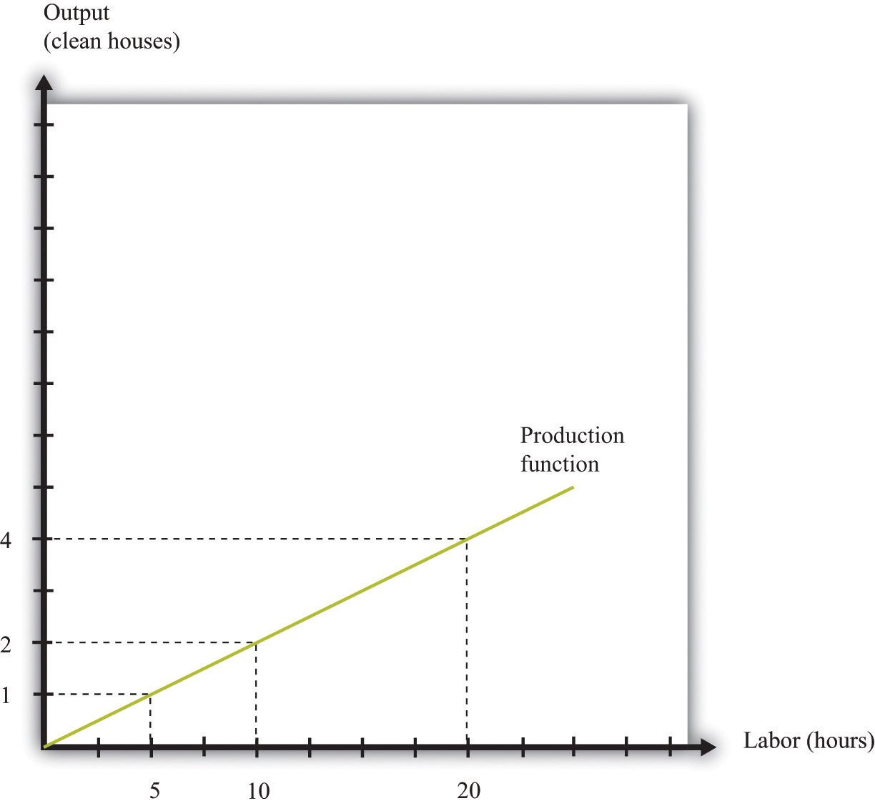
A production function shows the maximum amount of output produced, given a level of labor input.
The marginal product of laborThe amount of extra output produced from one extra hour of labor input. is the amount of extra output produced from one extra hour of labor input and is defined as
When the production function is linear, the marginal product of labor is constant. It is equal to the number we labeled productivity in our original production function.
In most cases, the marginal product of labor is not constant. To understand why, imagine you are managing a Starbucks outlet. You already have the machines to produce espresso, and you have lots of coffee beans on hand. You also have 500 square feet of space for making coffee and charging customers. But you still need labor. If you have no barista to operate the espresso machine, then you will have no output. If you hire one worker, you will be able to serve coffee to people. Adding the first worker will increase output considerably. However, that person must not only make the coffee but also clear the tables and handle the cash register. Adding a second worker to help with the register and clear tables will increase output even more. Now suppose you keep increasing the number of workers in the 500 square feet of space. After the third or fourth worker, they will start to bump into each other, and the barista will start to be very annoyed and unproductive. In other words, because one of your inputs—the amount of available space—is fixed, each additional worker contributes less and less to output. We call this the diminishing marginal product of laborThe idea that each additional hour of labor input contributes a smaller and smaller amount to output..
Table 9.2 "Production Function for Coffee with a Diminishing Marginal Product of Labor" is an example of a production function with a diminishing marginal product of labor. In creating this table, the labor input is changed while holding all other inputs (the size of the café, the number of espresso machines, etc.) fixed.
Table 9.2 Production Function for Coffee with a Diminishing Marginal Product of Labor
| Labor Input (Hours) | Output (Cups of Coffee) | Marginal Product of Labor |
|---|---|---|
| 0 | 0 | |
| 1 | 10 | 10 |
| 2 | 14.1 | 4.1 |
| 3 | 17.3 | 3.2 |
| 4 | 20 | 2.7 |
| 5 | 22.4 | 2.4 |
| … | ||
| 10 | 31.6 | 1.6 |
| 15 | 38.7 | 1.3 |
| 20 | 44.7 | 1.1 |
| 25 | 50.0 | 1.0 |
| 30 | 54.8 | 0.9 |
| 35 | 59.2 | 0.9 |
| 40 | 63.2 | 0.8 |
The marginal product of labor is shown in the third column. For the first few entries, you can calculate it directly from the table because you can easily determine how much output changes from one row to the next. For example, the marginal product of the third hour of labor is 17.3 – 14.1 = 3.2. Finding the marginal product of, say, the 40th unit of labor from the table is trickier because the table doesn’t tell us how much we can produce with 39 hours of labor. Looking back at the formula for the marginal product of labor, however, we can calculate it:
We illustrate this production function in Figure 9.7 "A Production Function with a Diminishing Marginal Product of Labor". Notice that while the slope of the production function is always positive, the slope decreases as the labor input increases.
Figure 9.7 A Production Function with a Diminishing Marginal Product of Labor
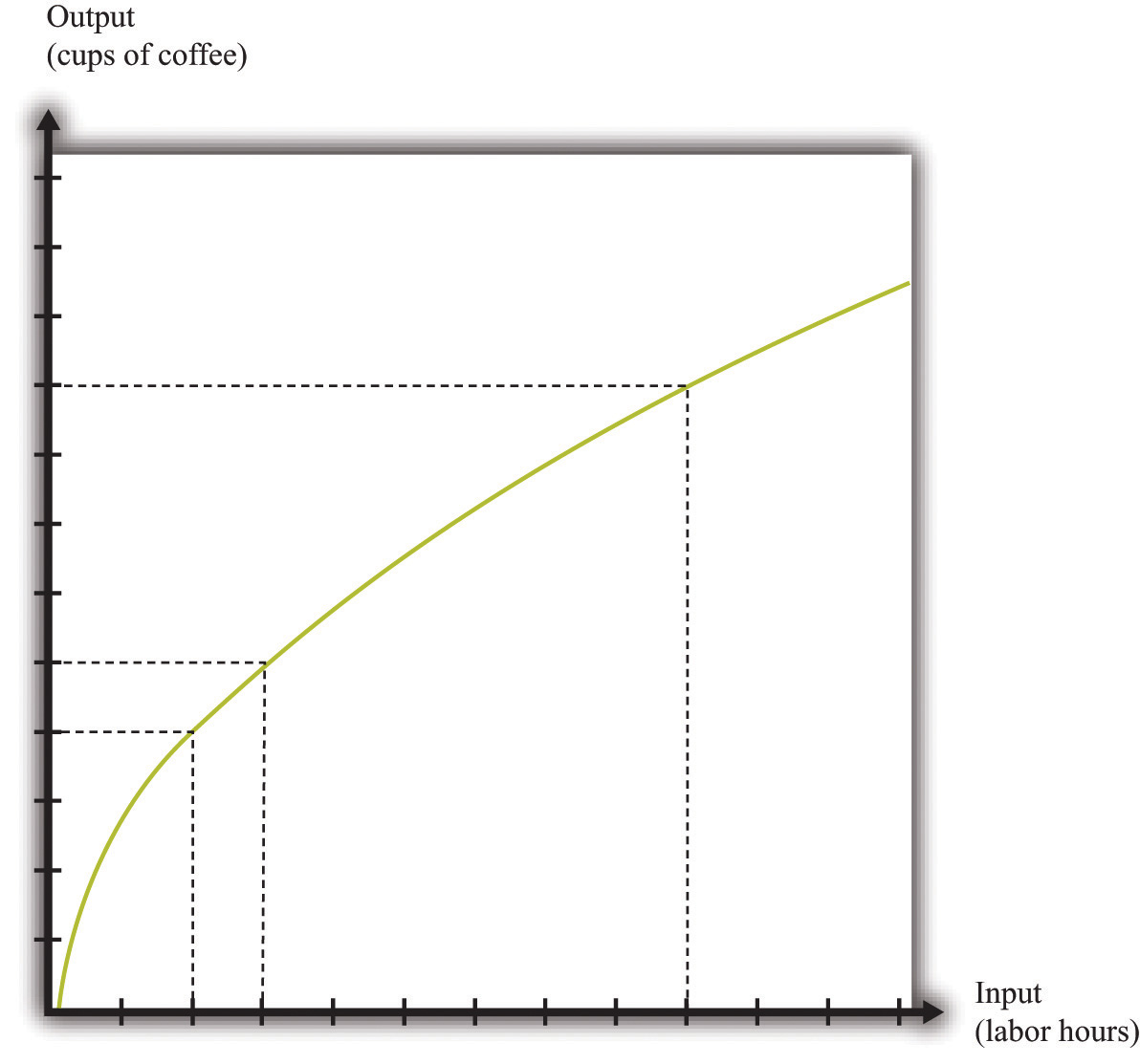
This production function exhibits diminishing marginal product of labor: as more labor is added to a firm, output increases at a decreasing rate.
Toolkit: Section 31.17 "Production Function"
The production function is a description of how much output a firm can produce as it varies its inputs. Typically, we suppose that the production function exhibits the following:
The first property means that adding more labor into production means more output—that is, the slope of the production function is positive. The second property explains how the marginal product of labor varies as labor input increases. Though the marginal product of labor is always positive, it will generally decrease as more labor is added to a production process. That is why the second property is called diminishing marginal product of labor. (It is technically possible that the marginal product of labor could even become negative. But because a firm would never pay for workers when they decrease output, we never expect to see a firm operating with a negative marginal product of labor.)
Now that we have a way of describing a firm’s ability to produce goods, we are well on our way to understanding how a firm produces output. This then allows us to understand how much it will cost a firm to produce different levels of output. Our next goal is to describe these costs. The total cost of producing some specified level of output represents the cost of acquiring all the inputs needed.
To see how this works, let us determine the costs for our earlier housecleaning example. Recall that the production function is
output = 0.2 × number of hours of labor input.Suppose that housecleaners can be hired at $10 per hour:
cost of one clean house = 5 hours × $10 per hour = $50.The cost of two clean houses is $100, the cost of three clean houses is $150, and so on.
More generally, suppose we take the linear production function and divide both sides by the level of productivity. We get
The cost of a single hour of labor is given by the wage. Thus we can write
This is the cost function of a firm, which is illustrated in Figure 9.8 "The Cost Function". Pay careful attention to the axes in Figure 9.6 "A Linear Production Function" and Figure 9.8 "The Cost Function". Figure 9.6 "A Linear Production Function" has hours of labor on the horizontal axis and output on the vertical axis. Figure 9.8 "The Cost Function" has output on the horizontal axis and costs (= labor hours × wage) on the vertical axis.
Figure 9.8 The Cost Function
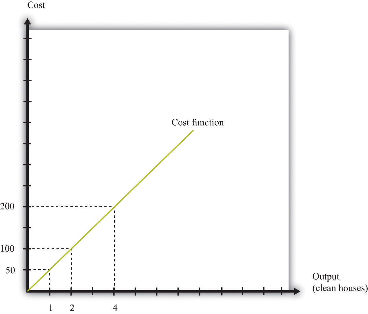
The cost function shows the cost of producing different levels of output.
The cost function in Figure 9.8 "The Cost Function" is linear. Because the production function has a constant marginal product of labor, the cost function displays constant marginal cost. What about the case in which the production function has a diminishing marginal product? Then additional labor provides less and less output. Turning this around, it follows that producing each additional unit of output requires more and more labor. We show this in Figure 9.9 "The Cost Function with a Decreasing Marginal Productivity of Labor". In this figure, the marginal cost is increasing, so the cost function gets steeper as we produce more output.
Toolkit: Section 31.14 "Costs of Production"
You can review the definition of marginal cost in the toolkit.
Figure 9.9 The Cost Function with a Decreasing Marginal Productivity of Labor
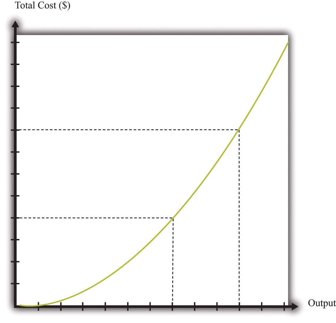
If a firm’s technology exhibits a diminishing marginal product of labor, the cost function will increase at an increasing rate.
We show the marginal cost curve in Figure 9.10 "The Marginal Cost Function". In this example, marginal cost is a straight line, but this need not be the case in general.
Figure 9.10 The Marginal Cost Function
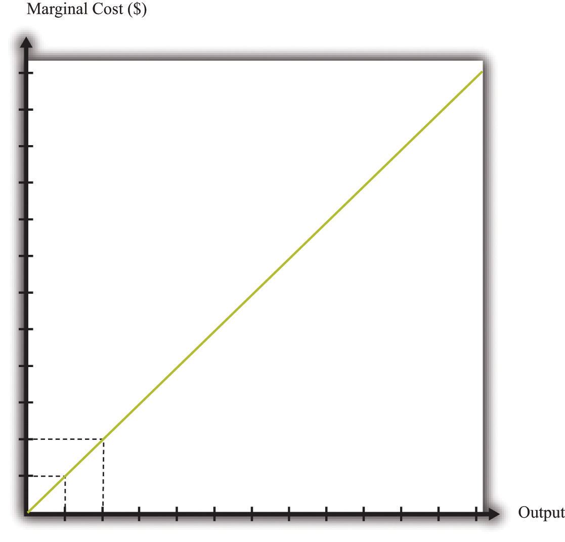
If a firm’s technology exhibits a diminishing marginal product of labor, then the marginal cost will increase as output increases.
Marginal cost depends on the following:
If the costs of inputs increase, then the marginal cost is higher is well. If the productivity of the inputs into the production function is higher, then the marginal cost is lower. In fact, marginal cost can be written as
We can see from this equation that when the marginal product of labor decreases, the marginal cost of production increases. We see also that an increase in the cost of inputs—in this case an increase in wages—leads to an increase in the marginal cost of production.
There is one issue that we are ignoring here. Firms typically have many different ways in which they can produce the same quantity of output. A firm might have a choice between two production processes: (1) a process that is simple and cheap to operate but wasteful of raw materials and (2) a process with recycling that uses fewer materials but is more complicated and costly to run. As another example, if a construction company needs to dig a ditch, it could employ 20 people and equip each with a shovel, or it could hire a single individual and a backhoe. Economists say that the first process is labor intensive because it requires a lot of labor relative to capital; they call the second process capital intensive because it requires a relatively large amount of capital.
In medium-sized or large firms, there is usually a specific functional area, called operations, that decides how to produce output. Operational decisions are governed in large part by technical or engineering considerations: what are the ways in which it is physically possible to transform inputs into the desired output? Operational decisions also have an economic component. Given that there may be many different ways to get the same final amount of output, which is the most cost effective? In economics, not surprisingly, we focus on the second of these questions and leave the first to engineers and other technical experts.
The basic principle is intuitive: operations managers tend to choose methods of production that economize on relatively expensive inputs. For example, much garment manufacture takes place in countries like China or Vietnam, where wages are low (that is, labor is relatively cheap). As a result, the production processes tend to be highly labor intensive, using a lot of workers relative to the amount of machinery. By contrast, garment manufacture in richer countries (where labor is much more expensive) tends to use methods of production that require fewer people and more machines.
We simply presume that the operations function of a firm is doing a good job and has succeeded in finding the cheapest way of producing the firm’s output, taking into account both the technical aspects of production and the costs of different inputs. When we talk about the cost function of a firm, therefore, we are assuming that it gives us the lowest cost for producing each given level of output.
We have now completed our discussion of the first decision that managers must make: how to produce output. The production function tells us what a firm needs in terms of inputs—in this case, labor—to produce a given level of output. The more output a firm wants to produce, the more labor it will hire and the more jobs it will create. The cost function tells us the cost of producing different levels of output, and the marginal cost function tells us the cost of producing additional output.
Marginal cost is the critical ingredient in the next decision made by managers, which is selecting a point on the demand curve. We can think of managers as either choosing the price and then selling the quantity demanded at that price or choosing the level of output and selling it at the price that the market will bear. In either case, they are picking the point on the demand curve whereThis decision of the firm is also covered in detail in Chapter 7 "Where Do Prices Come From?".
marginal revenue = marginal cost.We show this decision graphically in Figure 9.11 "Output and Price Decisions of a Profit-Maximizing Firm".
Figure 9.11 Output and Price Decisions of a Profit-Maximizing Firm
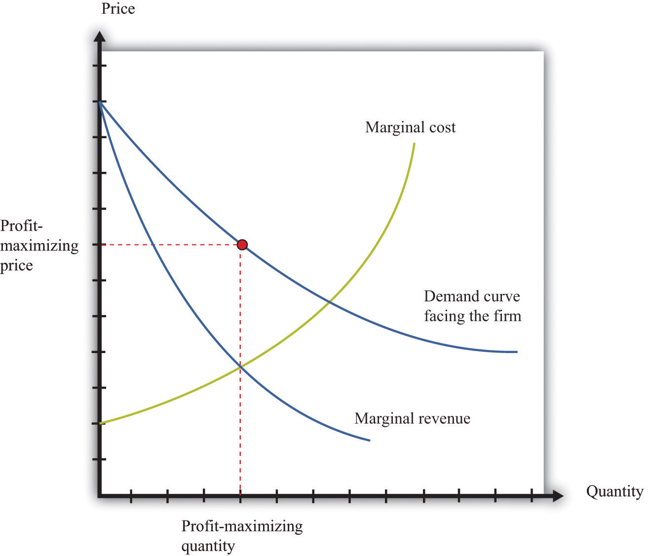
A profit-maximizing firm produces a quantity such that marginal revenue equals marginal cost, and the price is determined by the demand curve.
In our discussion of costs to this point, we have not specified whether we were talking about the nominal wage (that is, measured in dollars) or the real wage (that is, adjusted for inflation). The most important thing is being consistent. If we use the nominal wage when calculating our cost functions, then we end up with nominal costs. If we use the real wage, then we end up with real costs. And when we equate marginal revenue and marginal cost, we must be sure that we measure in nominal terms or real terms (not a mixture).
The distinction becomes important only when the general price level changes, so it is not central to our discussion here. When the price level is constant, we can always just suppose that it is equal to 1, in which case the nominal wage and the real wage are equal. Still, when we draw diagrams of the labor market, we typically put the real wage on the axis, so from here on we will explicitly suppose that we are measuring everything in real terms.
We can now explain labor demand by a firm. There are two steps:
We already know that the marginal cost of production depends on the real wage: decreases in the real wage lead to decreases in real marginal costs. Figure 9.12 "The Effect of a Change in Marginal Cost on a Firm’s Choice of Output and Employment" shows how a decrease in the real wage affects the output and price decision of a firm. As the real wage decreases, the marginal cost of an additional unit of output decreases, so a firm will choose to produce more output. The price will decrease because the firm must lower the price to sell the additional output.
Figure 9.12 The Effect of a Change in Marginal Cost on a Firm’s Choice of Output and Employment
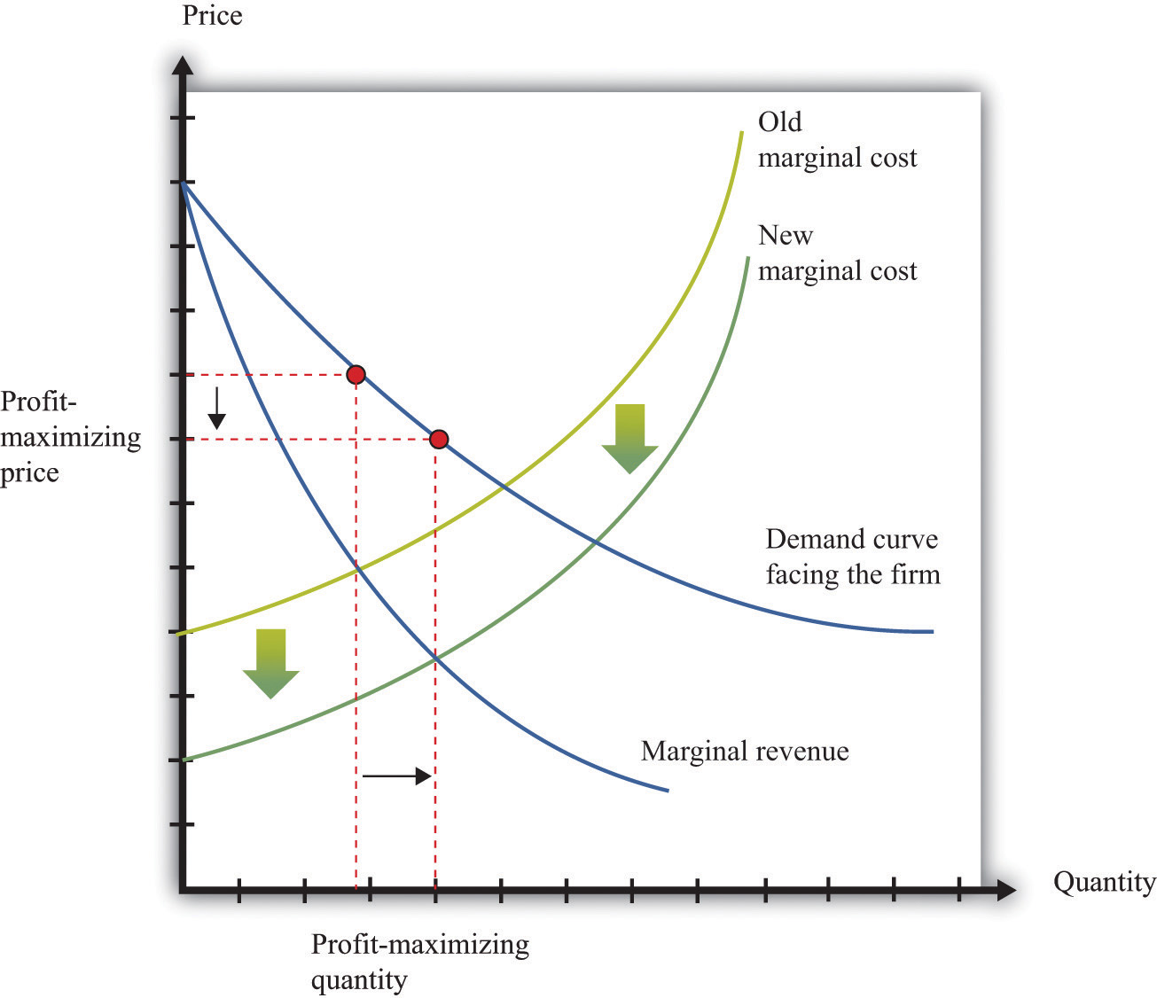
When the real wage decreases, marginal cost decreases, so the firm reduces price, increases output, and creates jobs.
Because a firm wants to produce more output, it will demand more hours of labor. In other words, a decrease in wages leads to an increase in the quantity of labor demanded. The resulting inverse relationship between the real wage and the amount of labor demanded is shown in Figure 9.13 "The Demand for Labor".
Figure 9.13 The Demand for Labor
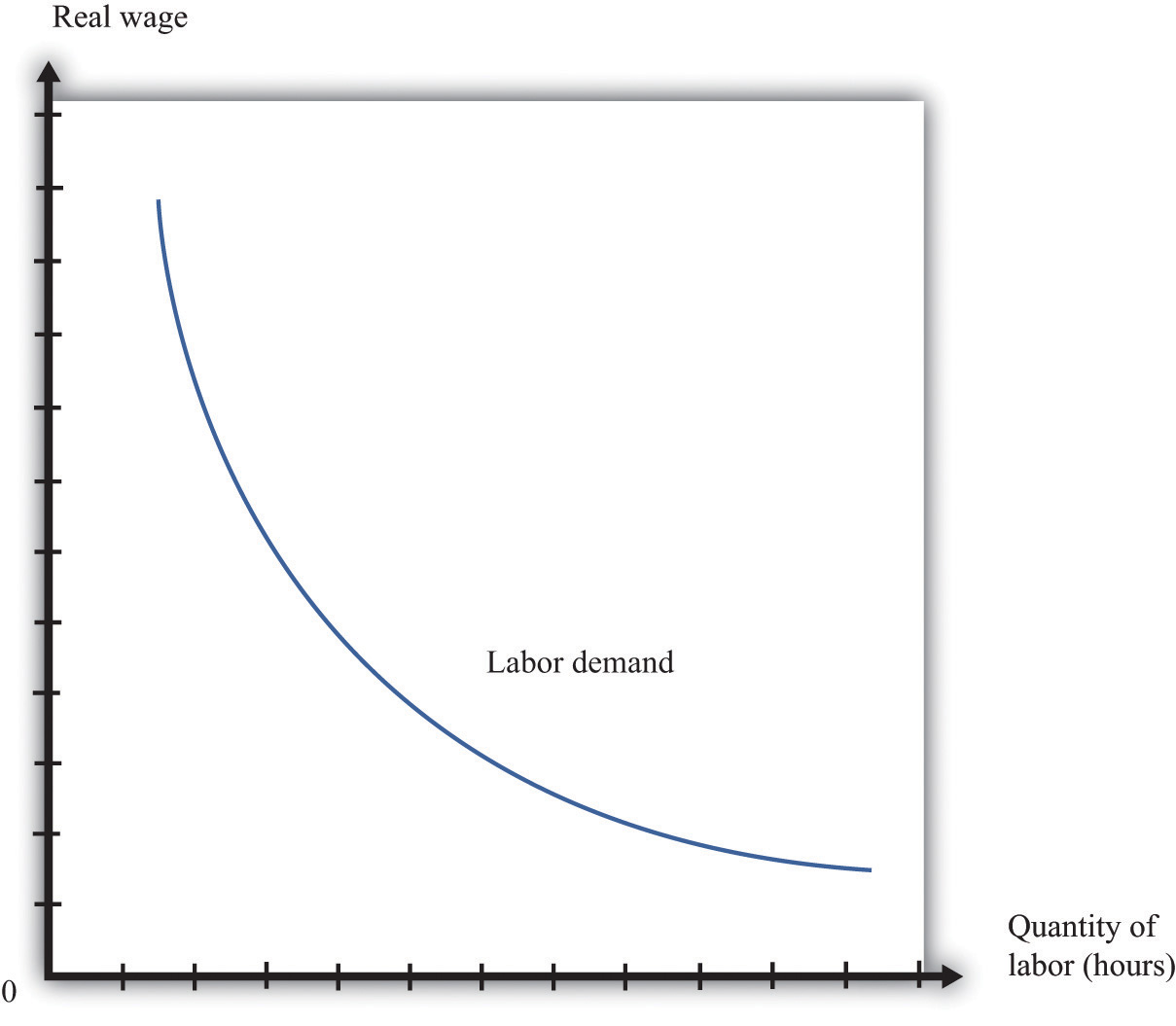
As the real wage increases, the demand for labor input decreases.
The labor demand curve for a single firm is downward sloping. This is true for every firm in the labor market. The market demand curve for labor is obtained by adding together the demand curves of individual firms. So the market demand for labor is downward sloping as well.
We can now connect our understanding of the labor market with the data on net job creation that we showed in Figure 9.3 "US Net Job Creation from 2000 to 2009". Based on what we have learned, there are three main reasons why jobs might be created or destroyed: (1) changes in the real wage, (2) changes in productivity, and (3) changes in demand.
Changes in the cost of labor are one reason firms create or destroy jobs. Decreases in the real wage lead firms to produce more output and hire more workers, thus creating jobs. Increases in the real wage cause firms to produce less output and lay off workers. Going deeper, we can ask why the real wage might change. The answer comes from looking back at Figure 9.4 "Labor Market Equilibrium". The real wage changes, causing a change in the quantity of labor demanded, if the labor supply curve shifts.
Population growth is one source of a shift in labor supply. As the number of workers in the economy grows, then total labor supply will shift. At a given wage, there will be more workers and hence the labor supply curve will shift to the right. Other things equal, this causes a decrease in the real wage.
Changes in labor market participation also shift the labor supply curve. A leading example of this is the increased participation of women in the labor market. In the United States, the fraction of women in the labor force rose from about 20 percent in 1950 to about 70 percent in 2000. Participation might also change because of workers’ expectations about the future state of the labor market. If you are worried you won’t have a job next year, you might want to work this year.
Changes in productivity—more precisely, in the marginal product of labor—work exactly like changes in the real wage. Remember that marginal cost depends on both real wages and productivity. If productivity increases, perhaps because a firm has upgraded its capital equipment, then marginal cost decreases. Firms will produce more output and hire more labor. The opposite is true if productivity decreases: in this case, firms will produce less and destroy jobs.
Over long periods of time, productivity in an economy increases. This increase in productivity is driven largely by technological advances: firms get better at producing goods and services and so are able to produce them more cheaply. As workers’ productivity increases, firms demand more labor at any given wage.
When a firm’s product becomes more desirable in the market, the demand curve that it faces shifts outward. This shift in demand typically leads to an outward shift in marginal revenue, inducing a firm to produce more output and demand more labor. We show this in Figure 9.14 "The Effect of a Change in Demand on a Firm’s Choice of Output and Employment": an outward shift of a firm’s demand curve typically leads to an outward shift in labor demand.
Figure 9.14 The Effect of a Change in Demand on a Firm’s Choice of Output and Employment
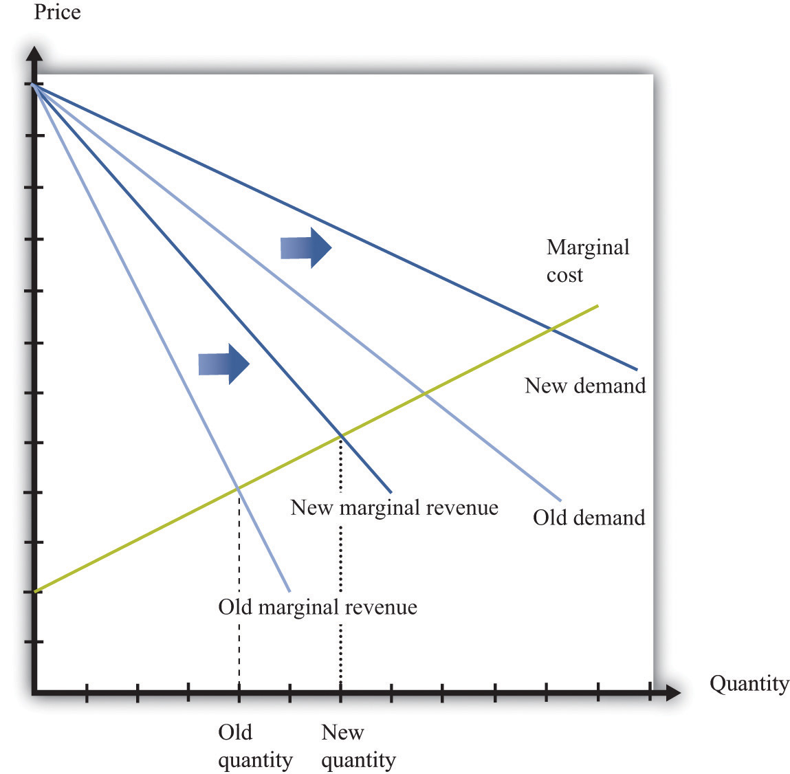
An increase in demand typically leads to an increase in marginal revenue, which in turn induces firms to produce more output and create jobs.
Marginal cost is defined as
We also know that
and
change in cost = wage × change in labor input.Show how you can use these three equations to derive the condition in the text that
So far we have been thinking about a firm simply changing the number of labor hours that it wants to plug into its technology. Such job creation and destruction takes place at individual firms all the time. Some firms see an increase in productivity and hire more workers. Other firms see reduced demand for their output and destroy existing jobs. The joint creation and destruction of jobs underlies the net job creation we displayed earlier in Figure 9.3 "US Net Job Creation from 2000 to 2009".
Yet the expansion and contraction of employment in existing plants is only one source of job creation and destruction. During an economic downturn, such as the severe recession that began in 2008, some firms closed factories, and other firms went completely out of business. For example, US automobile manufacturers, such as General Motors, responded to the decreased demand for cars by closing some of their existing manufacturing plants. This led to job destruction at these plants. At other times, when an economy is expanding, new firms enter into business and existing ones open new plants. Thus a complete picture of the job creation and destruction process requires us to understand the economics of entry and exit.
Only when the firm’s managers know how much the firm is going to produce, the price at which it will sell it, and the cost of producing that output can they figure out profits and decide whether it is sensible to be in business at all. This logic applies to both managers of firms that are already in business and entrepreneurs who are considering starting a business. Firms also apply this logic to parts of their operations—for example, a firm may want to decide whether to shut down an existing plant or open a new one.
If a firm that is already in business discovers that its profits are too small to justify its other costs, then it should exit the market, shutting down its operations completely. If an entrepreneur is contemplating starting a new firm and calculates that the profits it will earn justify the costs of setting up operations, then we say that a firm enters the market.
In the previous section, we explained how job creation and destruction take place as firms expand and contract. When Walmart comes to town, however, much more is going on. The opening of a new Walmart means that some new jobs are created. Against that, existing stores may be forced to close down completely. Now that we have looked at a firm’s price and output decisions, we are able to analyze entry and exit decisions.
Businesses do not stay around forever. At some point, they exit the market, destroying jobs in the process. Restaurants that were a big hit only a few years ago can quickly lose their luster and disappear from the scene. The same is true for many retail outlets. Manufacturing plants also close, taking jobs with them. Imagine, for example, that you own a small clothes retailing store. Then Walmart comes to your town. Now your customers have another place to buy their clothes, and you must decide whether to stay in business. You need to decide which is more profitable: staying in business or closing your business down and selling off any assets you possess.
To understand the factors influencing firm exit, we begin with a key distinction between different kinds of costs.
Toolkit: Section 31.14 "Costs of Production"
Costs that are the same at all levels of production are called fixed costs. Costs that vary with the level of production are called variable costs. As an accounting identity, the total costs of a firm are divided up as follows:
total costs = fixed costs + variable costs.Table 9.3 "Monthly Costs of Production" shows an example of fixed costsCosts that are the same at all levels of production., variable costsCosts that vary with the level of production., and total costsThe sum of fixed costs and variable costs. for your store. (To keep life simple, we treat all the different kinds of clothing you sell as if they were the same. Let us call them blue jeans.) The numbers in Table 9.3 "Monthly Costs of Production" are based on the following equation for costs:
total costs = 14,000 + 10 × quantity.Suppose your firm has fixed costs every month of $14,000. By definition, these fixed costs do not change as your level of output changes. Think of these as your overhead costs—for example, the cost of renting your retail space, utility bills, the wage of your sales clerk, and so on.
Table 9.3 Monthly Costs of Production
| Quantity | Fixed Costs ($) | Variable Costs ($) | Total Costs ($) |
|---|---|---|---|
| 0 | 14,000 | 0 | 14,000 |
| 1 | 14,000 | 10 | 14,010 |
| 2 | 14,000 | 20 | 14,020 |
| … | … | … | … |
| 200 | 14,000 | 2,000 | 16,000 |
| 400 | 14,000 | 4,000 | 18,000 |
| 600 | 14,000 | 6,000 | 20,000 |
| 800 | 14,000 | 8,000 | 22,000 |
| 1,000 | 14,000 | 10,000 | 24,000 |
| 1,200 | 14,000 | 12,000 | 26,000 |
| 1,400 | 14,000 | 14,000 | 28,000 |
| 1,600 | 14,000 | 16,000 | 30,000 |
| 1,800 | 14,000 | 18,000 | 32,000 |
| 2,000 | 14,000 | 20,000 | 34,000 |
| 2,200 | 14,000 | 22,000 | 36,000 |
| 2,400 | 14,000 | 24,000 | 38,000 |
By contrast, variable costs increase as the level of output increases. In this example, if output increases by one, variable costs increase by $10. You can think of this as the cost of purchasing your blue jeans from the wholesaler. For you, the cost of “producing”—that is, making available for sale—one more unit of output is $10. Figure 9.15 "Total Costs, Fixed Costs, and Variable Costs" graphs the data from this table. Notice that even if your firm produces no output at all, it still incurs fixed costs.
Figure 9.15 Total Costs, Fixed Costs, and Variable Costs
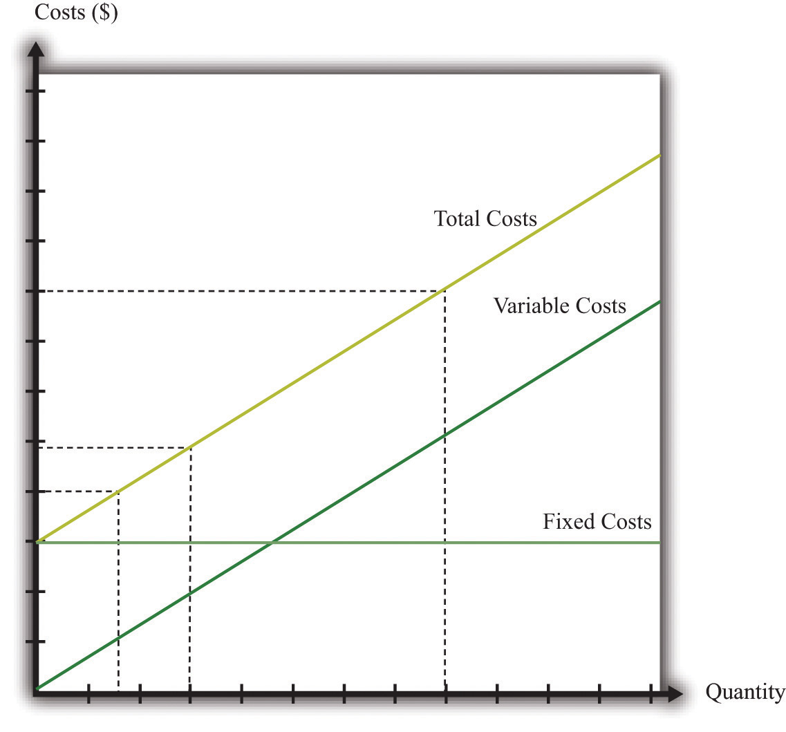
Fixed costs are the same at all levels of output. Variable costs increase as the quantity of output increases. Total costs equal fixed costs plus variable costs.
We are now ready to study the decision to continue in business or exit. You need to compare your revenues, defined as price times quantity, with the cost of running your business. Profit is the difference between revenues and costs, so
profit = total revenues − total costs = total revenues − variable costs − fixed costs.Table 9.4 Demand and Profit before Walmart Comes to Town
| Quantity | Price ($) | Total Revenues ($) | Variable Costs ($) | Fixed Costs ($) | Profits ($) |
|---|---|---|---|---|---|
| 0 | 30 | 0 | 0 | 14,000 | –14,000 |
| 200 | 29 | 5,800 | 2,000 | 14,000 | –10,200 |
| 400 | 28 | 11,200 | 4,000 | 14,000 | –6,800 |
| 600 | 27 | 16,200 | 6,000 | 14,000 | –3,800 |
| 800 | 26 | 20,800 | 8,000 | 14,000 | –1,200 |
| 1,000 | 25 | 25,000 | 10,000 | 14,000 | 1,000 |
| 1,200 | 24 | 28,800 | 12,000 | 14,000 | 2,800 |
| 1,400 | 23 | 32,200 | 14,000 | 14,000 | 4,200 |
| 1,600 | 22 | 35,200 | 16,000 | 14,000 | 5,200 |
| 1,800 | 21 | 37,800 | 18,000 | 14,000 | 5,800 |
| 2,000 | 20 | 40,000 | 20,000 | 14,000 | 6,000 |
| 2,200 | 19 | 41,800 | 22,000 | 14,000 | 5,800 |
| 2,400 | 18 | 42,550 | 24,000 | 14,000 | 5,200 |
The demand for your blue jeans is shown in the first two columns of Table 9.4 "Demand and Profit before Walmart Comes to Town". Looking at this table, your profit is at its highest when you set a price at $20 and sell 2,000 pairs of jeans. In this case, you earn $6,000 per month. Your revenues are enough to cover your variable costs and your fixed operating costsCosts incurred regularly during the normal operation of a business..
After Walmart comes to town, the demand for your jeans shifts inward because shoppers start going to Walmart instead. Now your demand is as shown in Table 9.5 "Demand and Profit after Walmart Comes to Town".
Table 9.5 Demand and Profit after Walmart Comes to Town
| Quantity | Price ($) | Revenues ($) | Variable Costs ($) | Fixed Costs ($) | Profit ($) |
|---|---|---|---|---|---|
| 0 | 26 | 0 | 0 | 14,000 | –14,000 |
| 200 | 25 | 5,000 | 2,000 | 14,000 | –11,000 |
| 400 | 24 | 9,600 | 4,000 | 14,000 | –8,400 |
| 600 | 23 | 13,800 | 6,000 | 14,000 | –6,200 |
| 800 | 22 | 17,600 | 8,000 | 14,000 | –4,400 |
| 1,000 | 21 | 21,000 | 10,000 | 14,000 | –3,000 |
| 1,200 | 20 | 24,000 | 12,000 | 14,000 | –2,000 |
| 1,400 | 19 | 26,600 | 14,000 | 14,000 | –1,400 |
| 1,600 | 18 | 28,800 | 16,000 | 14,000 | –1,200 |
| 1,800 | 17 | 30,600 | 18,000 | 14,000 | –1,400 |
| 2,000 | 16 | 32,000 | 20,000 | 14,000 | –2,000 |
| 2,200 | 15 | 33,000 | 22,000 | 14,000 | –3,000 |
| 2,400 | 14 | 33,600 | 24,000 | 14,000 | –4,400 |
In response to this decrease in demand, you should drop your price. Your profits are now maximized at $18. Unfortunately, at this price, you don’t earn enough to cover your fixed costs. Your profits are –$1,200 a month. Should you remain in business? The answer to this question depends on when you ask.
Suppose you ask this question just after you have paid your monthly fixed operating costs. During the course of a month, you should stay in business because you are earning enough revenues to cover your variable costs. As soon as it is time to pay your monthly fixed cost again, though, you should choose to exit and close down your store. In this case, you would engage in job destruction by firing your sales clerk.
In this simple example, it is easy to see exactly when and why you should exit. A more general rule for when to exit is as follows. You should exit if
discounted present value of expected future profits < value of recoverable assets.To make sense of this rule, we need to look at each part of it in turn.
Expected future profits. Even though your price has decreased this month, it might not stay low forever. Perhaps your customers will decide, after they have tried Walmart, that they prefer your store after all. It would then be foolish to close down your store immediately just because you fail to cover fixed costs in one month. This means you must make a decision in the presence of uncertainty: you don’t know for sure if your customers will come back, and if they do, you don’t know for sure that they will not go away again. As a simple example, suppose you think there is a 75 percent chance that the shift in your demand curve is permanent and a 25 percent chance that it will go back to its original position. Looking ahead and using the tool of expected value, you would calculate your expected profit as follows:
In this case, you still expect to make a small profit every month. Provided you were not too risk-averse, you would keep your store in business. Of course, after some months had gone by, you would probably have better information about whether your customers are truly coming back or not.
Toolkit: Section 31.4 "Choices over Time", and Section 31.7 "Expected Value"
You can review the meaning and calculation of discounted present value, expected value, and risk-aversion in the toolkit.
Our definition of fixed costs seems very straightforward. Unfortunately, it is not always easy to decide in practice whether a cost is fixed or variable. There are two main reasons for this:
In fact, if we take a very long time horizon and very large ranges of output, there are few costs that are truly fixed.
We use very similar reasoning to think about a firm’s decision to enter a market. When Walmart’s senior management team contemplates opening a new store, they compare the costs of entry against the (discounted present value of the) profit they expect to earn once they enter.
What are some of Walmart’s costs when it wants to open a new store?
You can probably think of many more. We call these Walmart’s entry costsThe one-time fixed costs that a firm must incur when establishing a business..
Toolkit: Section 31.14 "Costs of Production"
Entry costs are the one-time fixed costs that a firm incurs when establishing a business. The toolkit has more discussion of other kinds of costs.
Such costs of establishing a business can be very substantial. Notice, by the way, that entry costs are for the most part truly fixed costs. Walmart must incur these costs before it can let a single customer inside; these costs are fixed no matter how long the time horizon; these costs are largely independent of Walmart’s scale of operation.
The senior management team must also predict how much profit they expect the store to make. These forecasts are based on the idea that, once the store is opened, the store will set its prices and manage its operations to maximize its profits. Because the team will be uncertain about profits, they will need to use expected value calculations. They will also be counting on a profit flow for years if not decades and will need to use discounted present value calculations. Thus the appropriate decision rule for a firm is to enter ifIn Chapter 15 "Busting Up Monopolies", you will find an example of very similar economic reasoning. There we present a parallel rule for the situation where a firm is deciding whether or not to engage in innovation.
discounted present value of expected future profits > entry costs.A firm is more likely to enter if
Firms that enter markets know that it is possible that they will exit again in the future. Because their profit flow is uncertain, they recognize that there may come a point where they will judge it better to close down their operations. If they close down their operations, they may be able to sell off some of their existing assets. Therefore, when deciding to enter, managers also take into account the extent to which their assets are recoverable. If they are likely to be able to reclaim most of the value of their assets, then entry is more likely to be profitable even if demand turns out to be lower than expected.
Specifically, we can divide entry costs into sunk costsA cost that, once incurred, cannot be recovered. and recoverable costsA cost that, once incurred, can be recovered..
Toolkit: Section 31.14 "Costs of Production"
A sunk cost is a cost that, once incurred, cannot be recovered. A recoverable cost is a cost that, once incurred, can be recovered.
Looking back at our list of Walmart’s entry costs, we can see that many of these costs are sunk costs. All the planning and legal fees are completely tied to this store; if they end up not building the store, they cannot get any of the monies back. The building is a sunk cost as well. Other costs are at least partly recoverable. If they decide not to build the store, they can resell the land. If they have equipped the building with shelving and cash registers and then decide not to open the store, they can resell these assets or move them to another Walmart store instead.
Economic reasoning gives clear instructions about sunk costs: they should be irrelevant for any future decision. Whether it was a good or bad idea to build a store, any decisions made going forward should take into account only the future profitability of the store. For example, suppose that Walmart’s entry costs were $100 million, of which $30 million were recoverable. Suppose also that Walmart’s managers estimated the discounted present value of expected profits at $120 million and therefore decided to build the store. However, once it was built, they discover that they have badly overestimated demand. The managers revise their estimate of future profits by half to $60 million. They now regret having built the store; it was a bad investment. But they should still keep the store open because it is earning more than they could obtain by closing the store and selling its assets.
Even though the economic principle is clear, people frequently include sunk costs in their calculations instead of ignoring them. This is such a pervasive problem that it is given the name the sunk cost fallacyThe mistake of including sunk costs in future-looking decisions, even though they should properly be ignored..
Toolkit: Section 31.14 "Costs of Production"
The sunk cost fallacy is the mistake of including sunk costs in future-looking decisions, even though they should properly be ignored.
As we have seen, job creation and destruction occur because of the entry and exit of firms. Jobs are created when firms enter into an industry and destroyed when firms exit. Job creation and destruction also arise as a result of the hiring and firing decisions of existing firms. We have used the labor market as a device to help us understand these hiring and firing decisions.
If you have ever looked for a job, though, then you know there is more to the labor market than supply and demand. Several aspects of the way labor is traded do not fit neatly into this framework. Workers and firms devote time and money to finding one another: search is an important element of the job market. And wages are often determined by some type of bargaining process, perhaps between a single worker and a firm or between a firm and a union that represents many workers.
Internet job searches are now an established part of the way labor markets operate. If you are a worker looking for a job, you can go to a site like Monster.com (http://www.monster.com) or CareerBuilder.com (http://www.CareerBuilder.com) to search for vacancies posted by firms.The Department of Labor sponsors a website (http://www.careeronestop.org) filled with information, including compensation levels, for different occupations. Help with job search is available here as well. When you search on one of these sites, you are asked to provide information about the type of job you are looking for by providing the following:
In addition, you provide information about yourself, such as your work experience and education level. The search engine then provides a list of vacancies posted by firms matching these characteristics.
If there are potential matches for you, you are provided with a list of potential employers. Each will typically provide some information about the job. Sometimes this will include a salary range. These postings often include a description of the type of worker the firm is searching for, using phrases such as “team player,” “responsible,” “leadership skills,” or “people skills.” The next step is then up to you. Along with the job postings comes information about how to contact the firm. You can indicate your interest to the firm, and you may be called in for an interview. If that goes well, a job offer will follow. At this point, negotiation over compensation comes into play.
Eventually, you must decide whether or not to accept the job. What should you do? If you knew for sure that this was your dream job of a lifetime, the decision would be obvious: accept the job. But life is never that easy. In reality, you face considerable uncertainty over any job you are offered:
The first type of uncertainty has multiple dimensions. No matter how many brochures you read about a job, how many other workers you talk to, or how much time you spend watching someone at work, you still will not know everything about a job until you actually go to work. Even then, there are elements of a job that you will not know about until you have worked for many years. An example is promotion. When you consider a job, you will probably hear about opportunities for advancement if you stay with the firm. But whether or not you will be promoted is something that will be resolved in the future and is part of the uncertainty you face when you think about accepting a job.
The second type of uncertainty concerns the alternatives to the job you are considering. If you had a list of all possible jobs available to you, then you could consult that list and pick the best job. But, of course, there is no such list. Instead of being presented with a list, you have to search for a job. If you turn down the job you are offered today, you will not know for sure what job will be available to you tomorrow. Uncertainty over how to respond to a job offer is very important for some workers but less so for others. The difference is determined by how easy it is to change jobs. We can illustrate the point with two extreme examples.
The first case is a job that offers lifetime employment. If you accept this job, it is yours forever. You will never be fired and—let us suppose—you can never quit either. Given this situation and faced with a job offer, what would you do? Presumably the first thought that comes to your mind is “be careful.” You would not accept this job unless you were very sure it was a good match for you. If you are not sure, you should reject the job offer and search more.
The second case is a job that offers very short-term employment, on a week-by-week basis. If you accept this job, you are employed for the week; then you can choose to remain in the job (if it is still available) or leave to search for another one. Also, suppose that during your work time you can still keep an eye out for other jobs. It might be that you can check a computer that displays job ads, look at classified ads in the newspaper, or pass by a few shops advertising job openings during lunch. If you are offered this second type of job, there is no need to be very selective. Your employment is very temporary, and it is easy to change jobs.
The first kind of job is more descriptive of professional positions available to highly skilled workers, where employers are very selective about the type of person they hire. For these types of individuals, searching and changing jobs can be very lengthy and expensive. If they accept a job, it had better be right for them. The second kind of job is one you might be more familiar with as a student—a short-term job such as waiting tables, working as a secretarial temp, or selling in a retail outlet.
The existence of Monster.com and similar search engines makes clear that the trade of labor services is quite different from the trade of, say, US government bonds. The return on a bond is the same regardless of who owns it. But the match between a firm and a worker is special. No two jobs are the same, and no two workers are the same. Also, if you want to buy a US government bond, you can simply call a broker to buy one for you. But if you run a restaurant and want to hire a worker with some very special skills in a particular location, there is no obvious person to call or place to go.
There are three stages of search and bargaining:
These three elements correspond to the stages you might encounter when you look for a job. First, there is time spent looking for job opportunities. This might involve a recruiting program or search on the Internet. Once you have found a job opening, there is normally a second stage: an interview process. You will typically be interested in the characteristics of the job (such as wages, hours, benefits, promotion possibilities, and job security), and the firm will be interested in your characteristics (such as skills, experience, and trustworthiness). If both you and the firm think that the match is a good one, then the process moves to a third and final stage of bargaining to determine the compensation you will receive.
We suppose that the bargaining process between a worker and a firm is very simple. The firm makes a take-it-or-leave-it offer. In other words, the firm gives the terms of its offer, including the compensation package and the working conditions, and the worker can then either accept or reject this offer. We also suppose that the offer can be summed up in terms of wages.
To see how this works, imagine that there are two firms each offering jobs at $10 per hour. One firm provides very flexible working hours, while the other requires you to work from 10 p.m. to 6 a.m. and sometimes on the weekend. The first job is evidently more desirable than the second one. If you would be willing to pay $4 an hour for the flexibility of the first job, then it is as if the second firm was offering a job at $6 per hour.
Once a worker has a wage offer in hand, should that person accept or reject it? The answer comes from balancing the benefits of having a job (and therefore a wage) right now versus waiting for another job to come along in the hope that it will pay a higher wage. To see how a worker would make this choice, here is a simple numerical example.
Suppose a worker gets a job offer of $1,000 per week. Then the decision is easy: accept that job. The more difficult case is when the worker gets an offer of $500 per week. By accepting this job, the worker gets $200 more than with unemployment insurance. But accepting the job also has an opportunity costWhat you must give up to carry out an action.. It means that the worker loses out on the chance of getting the higher paying job next week. So what should the worker do?
If you think about this problem, you will probably realize that the answer depends on how likely the worker is to get the better job by waiting. If most of the available jobs are the ones that pay $1,000 per week, then it is likely to be worth waiting. On the other hand, if most of the jobs pay only $500 a week, then the worker might have to wait a long time for the better job, so it is likely better to accept the one that pays $500 a week. More generally, in a world where there are lots of different jobs paying lots of different wages, the best thing for the worker to do is to pick something we call the reservation wageThe lowest wage that a searching worker will accept.. Workers can follow this rule:
If a worker and a firm meet and determine that the match is good, then they proceed to determine wages. There are two ways in which this might happen.If you read Chapter 6 "eBay and craigslist", you will see some close parallels between the mechanisms we discuss here and the ways in which a buyer and a seller may agree on a price. One possibility is the one we just discussed. Firms post vacant jobs and at the same time advertise the wage. If a worker qualifies for the job, then that worker will accept the job if the wage exceeds the reservation wage.
There can also be bargaining between a worker and a firm. A firm will make a profit based on the difference between the marginal product of hiring the extra worker and wages paid to the worker. So a firm will choose to hire the worker as long as the wage is below the marginal product of labor. This is a firm’s valuation of the job. A worker will be willing to take a job as long as the wage exceeds the reservation wage. This is a worker’s valuation of the job. In Figure 9.16 "The Valuation of a Job" we show both.
Figure 9.16 The Valuation of a Job
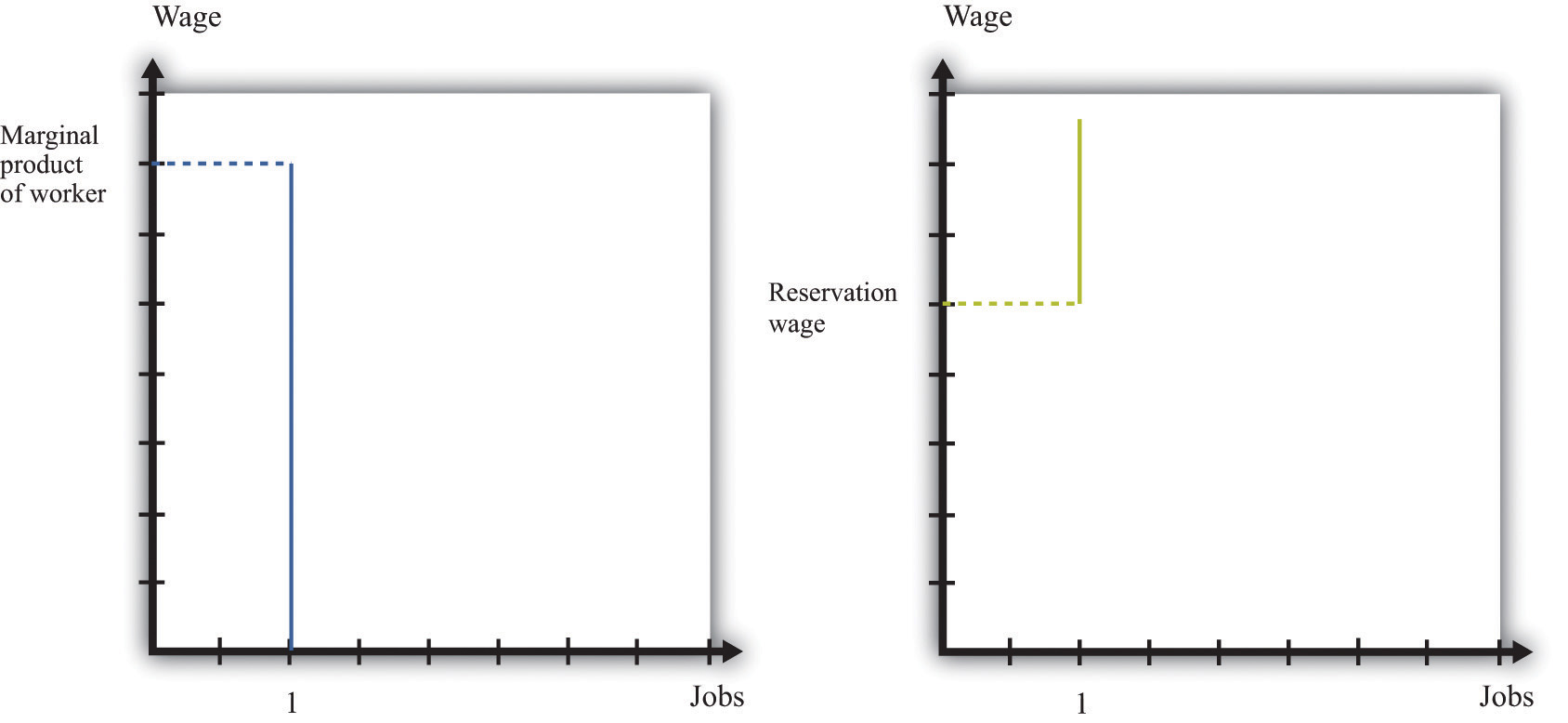
A firm follows the decision rule: “Offer the job if a worker’s marginal product exceeds the wage.” A worker follows the decision rule: “Accept the job if the wage exceeds the reservation wage.”
As long as the marginal product of labor for a worker is higher than a worker’s reservation wage, there is something to gain by employing a worker. The match is potentially a good one. But how will these gains be split? The answer depends on the relative bargaining power of a worker and a firm, which in turn depends on the information that they each possess.
As an example, suppose that a firm knows a worker’s reservation wage and can make a take-it-or-leave-it offer. It would then offer a real wage slightly above the worker’s reservation wage. The worker would accept the job, and all the surplus from the employment relationship would flow to the firm. At the other extreme, suppose that a worker knows his marginal product at the firm, so the worker can make a take-it-or-leave-it offer. Then the worker will offer to work at a real wage slightly below his marginal product. The firm would accept the offer, and all the surplus of the employment relationship would flow to the worker.
Another source of bargaining power for a worker is the other options available to him. If a worker comes into a negotiation with a good job offer from another firm in hand, then this will increase his reservation wage.
Workers can also enhance their bargaining power by negotiating together. Firms typically have many workers. Sometimes these workers group together, form a union, and bargain jointly with a firm. When workers organize in this way, they generally have more bargaining power because they can threaten to strike and shut down the firm. In this way, unionized workers get more of the surplus from their jobs.
In reality, workers don’t know their exact marginal product and firms don’t know the exact reservation wage of their workers. Not surprisingly, bargaining in such situations is more complicated to analyze. Sometimes, gains from trade are not realized. Suppose, for example, that a worker’s reservation wage is below his marginal product. But a firm, thinking that a worker’s reservation wage is really low, makes the worker a very low wage offer. If this wage offer is below the worker’s reservation wage, then the worker will decline the offer and search again—despite the fact that there were gains to trade. Unfortunately, private information prevented the firm and the worker from realizing these gains.
The final element in the search process is the vacancies posted by firms. You can see these vacancies on Monster.com, in the newspaper, and in magazines. Vacancies are costly to post, and it is expensive to evaluate workers. They are the analogy on a firm’s side to the costly search on a worker’s side.
You can think of a firm’s decision of posting vacancies as being very similar to the labor demand for a firm. Firms want to expand output and thus post more vacancies whenever the marginal revenue of selling an extra unit of output increases relative to marginal cost. This could happen, for example, if the demand curve faced by a firm shifts outward. To expand output, the firm needs to hire more workers. It does so by posting vacancies, interviewing workers, and eventually bargaining with the best qualified ones to fill the open positions.
We noted earlier that labor demand also depends on wages: as the real wage decreases, a firm’s real marginal cost decreases, so it will want to hire more workers and expand output. When we think of search and bargaining, say through Monster.com, there is no “market wage” that a firm takes as given. Instead, the wage comes from a bargain between a worker and the firm. But the wage that is eventually agreed on will depend on the outside options of workers and firms. As the prevailing wage in the market decreases, a firm will be able to hire workers at a lower wage and will choose to post more vacancies and expand its workforce.
Governments are very interested in job creation. A political leader whose economy loses a large number of jobs without creating new ones is unlikely to be reelected. On a local level, state and local governments compete fiercely to have firms locate in their region by offering lucrative tax reductions. This is seen as a way to create jobs in the local economy. We now examine some of these policy interventions and trace out their implications, focusing on three policies: restrictions on closing plants, policies that promote small businesses, and trade policies.
In the United States, if you want to close a factory, you do not have to have approval of the government, but an act of Congress—the Worker Adjustment and Retraining Notification ActUS Department of Labor, “Other Workplace Standards: Notices for Plant Closings and Mass Layoffs,” elaws Employment Law Guide, accessed March 14, 2011, http://www.dol.gov/compliance/guide/layoffs.htm.—requires you to announce your intentions ahead of time. According to the US Department of Labor, “The Worker Adjustment and Retraining Notification Act (WARN) protects workers, their families, and communities by requiring employers to provide notification 60 calendar days in advance of plant closings and mass layoffs.”US Department of Labor, The Worker Adjustment and Retraining Notification Act (WARN), accessed January 22, 2011, http://www.dol.gov/compliance/laws/comp-warn.htm.
This law was passed in 1988 during a time of higher than average unemployment in the United States. Similar restrictions apply in some European countries, such as Spain and France. You cannot simply close an unproductive plant; employees must be given advance notice, and government approval may be required. Such restrictions on plant closings are intended to reduce job destruction. After all, if you make something more expensive to do, then less of it will be done. If it becomes more expensive to close plants, then fewer jobs will be destroyed by the exit of plants.
Economists point out, however, that the incentives of such policies are complicated and go beyond the effects on job destruction. To see why, think about our earlier discussion of entry and exit. When a firm decides to enter into an industry, it compares the profit flow from operating to the entry cost. When a firm thinks about the profits it will earn if it enters, it recognizes that if the demand for its product disappears, it can exit and thus avoid periods of negative profits. But if you take this option to exit a market away from a firm, then the value of entering an industry will decrease. Fewer firms will enter, and fewer jobs will be created. Thus laws that make it costly to close plants will also reduce job creation. The effect on net job creation is unclear.
Started in the 1950s, the Small Business Administration (SBA; http://www.sba.gov) is a US government agency whose goal is to protect and promote small businesses. Small firms obtain preferential treatment in terms of taxes, regulation, and other policies. Part of the argument in favor of promoting and protecting small businesses is the view that job creation is centered on these firms. According to the SBA website, small businessesSee http://www.sba.gov/sites/default/files/files/leg_priorities112th.pdf.
So it appears that small businesses are critical to an economy.
We must remember that these are indeed small firms, however. Suppose there were 5 firms in an economy. Four of them have 2 workers, and the fifth has 92 workers. The typical firm then has 2 workers: 80 percent of the firms in this economy have 2 or fewer workers. From the perspective of workers, though, things are rather different. Ninety-two percent of the workers are employed by the single large firm. If you ask workers how many employees are in their firm, the typical worker will say 92. Most firms have few workers, but most workers are employed by the large firm.
This is not far from the reality of the US economy, where much economic activity (employment and output) is centered on relatively few firms. A recent study of about 5.4 million businesses found that 182,000 of them operate multiple units. Dividing 182,000 by 5.4 million, we learn that these larger firms are less than 4 percent of the total number of firms. But they account for about 61 percent of the revenue of the business sector of the economy. So most firms are relatively small, but those that are large are huge compared to the rest.Steven J. Davis et al., “Measuring the Dynamics of Young and Small Business: Integrating the Employer and Non-employer Universes” (NBER Working Paper 13226, 2007), accessed January 30, 2011, http://www.nber.org/papers/w13226.
Davis, Haltiwanger, and Schuh point out that “large firms and plants dominate the creation and destruction of jobs in the manufacturing sector.”See Steven J. Davis, John C. Haltiwanger, and Scott Schuh, Job Creation and Destruction (Boston, MA: MIT Press, 1998), chap. 7, sect. 4. Larger firms and plants both destroy and create more jobs. For example, at a job destruction rate of 10 percent a year, a small firm of 50 workers will destroy 5 jobs, while a large plant with 1,000 workers will destroy 100 jobs. So even if the job creation and destruction rates are higher for small firms, this does not necessarily mean that these small entities create and destroy more jobs than large firms do.
This is not to say that small firms are unimportant. Most of the large firms in the economy started small. Likewise, all the older, more successful firms were once young firms. So any impact the SBA has on either small or young firms will influence these firms as they age and grow. However, the rationale for the SBA is not completely clear. Normally, government interventions are based on the idea of either correcting some problem with the operation of free markets or redistributing resources. It is not clear whether the SBA fulfills either of these roles.
Job creation and destruction are also affected by things that happen outside US borders. The removal of trade barriers allows countries to benefit more fully from the gains from trade. But in the process, some jobs are destroyed, while others are created.
Job destruction frequently takes center stage during debates on trade policy. In the early 1990s, for example, the United States was contemplating a reduction in trade barriers with its neighbors—Canada and Mexico—through negotiation of the North American Free Trade Agreement (NAFTA). Ross Perot, a third-party candidate for the US presidency in 1992 and 1996, was extremely critical of NAFTA. His focus was on job destruction, and he was famous for forecasting “a giant sucking sound” as employment opportunities moved from the United States to Mexico in response to NAFTA.
The loss of some jobs from a reduction in trade barriers is part of the adjustment one would expect. For countries to reap the gains from trade brought about by the removal of trade barriers, production patterns across countries must change. That process leads to job destruction and creation. Firms that used to produce certain goods in one country exit, as firms in other countries start to produce those goods instead. Workers at the exiting firms will certainly lose their jobs, but other jobs are created in the economy at the same time.
NAFTA was implemented in January 1994. More than 15 years later, it is still difficult to say exactly what the effects were and will be of NAFTA. Economics is not a laboratory science. It is not possible to subject the economies of Canada, Mexico, and the United States to this reduction in trade barriers, holding everything else the same. Instead, we have to look at data from before and after 1994 to try to infer the effects of NAFTA. But of course many other economic factors have also changed over this period. In parts of the United States where manufacturing jobs have been lost over the last 15 years, there is a tendency to hold NAFTA responsible. In fact, there is little evidence that NAFTA led to net job destruction.
What has happened over the last decade is that the US manufacturing sector has been exposed to increased competition from other countries, most notably China. It is this trade that has had a bigger impact on US manufacturing. At the same time, this has meant that NAFTA has been less of a success story for the Mexican economy than was predicted and hoped, as US consumers have purchased very cheap goods from China rather than Mexico.
During election season in the United States, the adverse effects of trade on jobs are often talked about extensively. In the 2008 Michigan presidential primary election, for example, candidates offered different ways in which they claimed they would help the automobile industry and bring more jobs to the Michigan economy. In the South Carolina primary in the same year, job losses in the textile industry received lots of attention. One large textile manufacturer in the region, Swift, had been cutting jobs steadily and was closing up, apparently planning to move production to South America. Individuals who lost their jobs due to this closing reported that they experienced a period of unemployment as they searched for a new job. Some found new jobs, either in an automobile assembly plant or working on optic fibers. Others moved from working in manufacturing to services. This is job creation and destruction in action. It happens all the time, all across the world.
Viewed abstractly, job creation and destruction are healthy processes for an economy. Through the process of job creation and destruction, workers are induced to move from less productive to more productive jobs. Such movement enhances the overall productivity of an economy. From the perspective of individual workers, however, the process looks very different. Job destruction means that people lose their jobs, which are a source of income and perhaps also of pride and dignity. They may have to spend some period of time unemployed, and they may lose important benefits, such as health insurance. They may have to relocate in search of jobs that are being created elsewhere; such relocation can be difficult and costly.
In sum, although the productivity of an economy as a whole may increase, this need not translate into improvements for workers who lose their jobs. Some find higher-paying jobs, but others, particularly those with few skills, see their wages decrease. One of the big challenges faced by governments and policymakers is to encourage the efficient reallocations of workers while minimizing the individual hardships that workers confront.
Spreadsheet Exercise
Economics Detective