Newspaper headlines around the world in 2008 asked whether the world’s economies were heading for another “Great Depression.” Long-past economic history suddenly captured the attention of economists, journalists, and others. But what was this event and why—even though it occurred the best part of a century ago—does it still hold such a prominent place in our economic memories?
In the early 1930s, instead of benefiting from economic growth and improved standards of living, people witnessed a huge decline in the level of economic activity. There was great economic hardship: large numbers of families struggled to obtain even basic food and shelter. Some sense of the desperation during these times can be found in oral histories. Here, for example, is one person’s story of what it was like trying to find a job:
I’d get up at five in the morning and head for the waterfront. Outside the Spreckles Sugar Refinery, outside the gates, there would be a thousand men. You know dang well there’s only three or four jobs. The guy would come out with two little Pinkerton cops: ‘I need two guys for the bull gang. Two guys to go into the hole.’ A thousand men would fight like a pack of Alaskan dogs to get through there. Only four of us would get through. I was too young a punk.See Studs Terkel, Hard Times: An Oral History of the Great Depression (New York: Pantheon Books, 1970), 30.
The personal suffering is less apparent in the figure below, but this picture does reveal the extraordinary nature of those times. It shows real gross domestic product (real GDP) in the United States from 1890 to 1939. Three things stand out. First, the level of economic activity grew substantially during this half century. This is normal: economies typically grow over the long haul, becoming more productive and producing more output. Second, although the level of US economic activity grew substantially over this half century, there were many ups and downs in the economy during the late 19th century and early 20th century. Third—and most important for our purposes—the period from 1929 to 1937 stands out from the rest. This was not a minor blip in economic activity; the US economy suffered a collapse that persisted for many years. At the same time, unemployment climbed to a staggering 25 percent in 1933—one out of four people was unemployed—compared to a rate of only 3.2 percent in 1929.
Figure 22.1 US Real GDP, 1890–1939
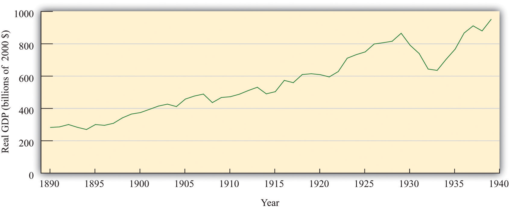
Real GDP increased considerably between 1890 and 1939, but the Great Depression of the early 1930s is a striking exception.
Source: Data from “What Was the U.S. GDP Then?,” Measuring Worth, accessed August 22, 2011, http://www.measuringworth.org/datasets/usgdp/result.php.
The United States was not the only country to experience such hard economic times in this period. Many other countries, such as the United Kingdom, Canada, France, Germany, and Italy also saw their economic progress reversed for a period of years. The Great Depression, as this economic cataclysm came to be called, was a shock to the economists of the day. Prior to that time, most economists thought that, though economies might grow fast in some years and decline slightly in others, prolonged unemployment and underutilization of resources was impossible. The Great Depression proved this view to be erroneous and eventually led to a fundamental change in the way in which economists thought about the aggregate economy. The idea that the economy was naturally stable was replaced with a view that severe economic downturns could recur at any time.
Along with this change in thinking about the economy came a change in attitudes toward macroeconomic policy: economists began to believe that the government could play an active role to help stabilize the economy, perhaps by increasing government spending in bad times. Prior to the Great Depression, nobody even thought that the government should try to keep the economy stable. Both Democrats and Republicans in the 1932 election advocated less government spending because government revenues had fallen. Yet, by the end of the 1930s, the United States and other countries had adopted the view that active policy measures were useful or even essential for the proper functioning of economies.
Three-fourths of a century later, these events are part of economic history. Few people still alive experienced those terrible years directly, yet the time remains part of our collective memory. Above all, we need to know what went wrong if we hope to ensure that such punishing times do not come again. Indeed, the world economy recently suffered the most severe recession since the 1930s, and it is unclear at the time of this writing how long or how bad the current crisis will be. The insights of the economists who explained the Great Depression are still at the heart of today’s discussions of economic policy. Understanding what happened to the economy in the 1930s is more than an exercise in economic history; it is essential for understanding modern macroeconomics. We want to know—
What caused the Great Depression?
We begin by looking at some facts about the Great Depression and the boom that preceded it. Our goal is to see if we can develop a good explanation of these facts. The most fundamental defining feature of the Great Depression was the large and sustained decrease in real GDP. In the figure below, which shows the circular flow of income, reminds us that real GDP measures both production and spending.
Figure 22.2 The Circular Flow of Income
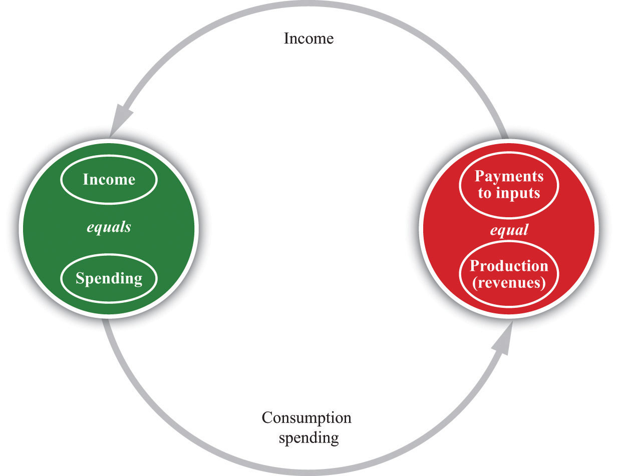
GDP measures the production of an economy and total income in an economy. We can use the terms production, income, spending, and GDP interchangeably.
It follows that during the Great Depression, both output and spending decreased. Perhaps it is the case that production in the economy declined for some reason, and spending decreased as a consequence. Or perhaps spending declined for some reason, and production decreased as a consequence. We examine two approaches to the Great Depression, based on these ideas. One sees the root cause of the Great Depression as a decline in the productive capabilities of the economy, meaning that firms—for some reason—were unable to produce as much as they had before. This then led to decreased spending. The other approach sees the root cause of the Great Depression as a decline in spending, meaning that households and firms—for some reason—decided that they wanted to purchase fewer goods and services. This then led to decreased production.
We look at each explanation in turn. We investigate which inputs contributed the most to the decrease in output and also look at what happened to the different components of spending. This more careful look at the data helps us to evaluate the two competing theories of the Great Depression. We conclude by examining the implications for economic policy and considering what policies were actually conducted at the time of the Great Depression.
After you have read this section, you should be able to answer the following questions:
We begin with some facts. Table 22.1 "Major Macroeconomic Variables, 1920–39*" shows real gross domestic product (real GDP)A measure of production that has been corrected for any changes in overall prices., the unemployment rateThe percentage of people who are not currently employed but are actively seeking a job., the price levelA measure of average prices in the economy., and the inflation rateThe growth rate of the price index from one year to the next. from 1920 to 1939 in the United States. Real GDP measures the overall production of the economy, the unemployment rate measures the fraction of the labor force unable to find a job, the price level measures the overall cost of GDP, and the inflation rate is the growth rate of the price level.
Table 22.1 Major Macroeconomic Variables, 1920–39*
| Year | Real GDP | Unemployment | Price Level | Inflation Rate |
|---|---|---|---|---|
| 1920 | 606.6 | 5.2 | 11.6 | |
| 1921 | 585.7 | 11.7 | 10.4 | −10.3 |
| 1922 | 625.9 | 6.7 | 9.8 | −5.8 |
| 1923 | 713.0 | 2.4 | 9.9 | 1.0 |
| 1924 | 732.8 | 5.0 | 9.9 | 0.0 |
| 1925 | 748.6 | 3.2 | 10.2 | 3.0 |
| 1926 | 793.9 | 1.8 | 10.3 | 1.0 |
| 1927 | 798.4 | 3.3 | 10.4 | 1.0 |
| 1928 | 812.6 | 4.2 | 9.9 | −4.8 |
| 1929 | 865.2 | 3.2 | 9.9 | 0.0 |
| 1930 | 790.7 | 8.9 | 9.7 | −2.0 |
| 1931 | 739.9 | 16.3 | 8.8 | −9.3 |
| 1932 | 643.7 | 24.1 | 8.0 | −9.1 |
| 1933 | 635.5 | 25.2 | 7.5 | −6.3 |
| 1934 | 704.2 | 22.0 | 7.8 | 4.0 |
| 1935 | 766.9 | 20.3 | 8.0 | 2.6 |
| 1936 | 866.6 | 17.0 | 8.1 | 1.3 |
| 1937 | 911.1 | 14.3 | 8.4 | 3.7 |
| 1938 | 879.7 | 19.1 | 8.2 | −2.4 |
| 1939 | 950.7 | 17.2 | 8.1 | −1.2 |
| *GDP is in billions of year 2000 dollars (Bureau of Economic Analysis [BEA]). The unemployment rate is from the US Census Bureau, The Statistical History of the United States: From Colonial Times to the Present (New York: Basic Books, 1976; see also http://www.census.gov/prod/www/abs/statab.html). The base year for the price index is 2000 (that is, the index equals 100 in that year) and comes from the Bureau of Labor Statistics (BLS; http://www.bls.gov), 2004. | ||||
Looking at these data, we see first that the 1920s were a period of sustained growth, sometimes known as the “roaring twenties.” Real GDP increased each year between 1921 and 1929, with an average growth rate of 4.9 percent per year). Meanwhile the unemployment rate decreased from 6.7 percent in 1922 to 1.8 percent in 1926. Real GDP reached a peak of $865 billion in 1929. This number is expressed in year 2000 dollars, so we can compare that number easily with current economic data. In particular, if we divide by the population at that time, we find that GDP per person was the equivalent of about $7,000, in year 2000 terms. Real GDP per person has increased about fivefold since that time.
Toolkit: Section 31.21 "Growth Rates"
You can review growth rates in the toolkit.
The Great Depression began in late 1929 as a recession not unlike those experienced previously—a decrease in GDP from one year to the next was common—but it rapidly blossomed into a four-year reduction in economic activity. By 1933, real GDP had fallen by over 25 percent and was only $636 billion. At the same time, unemployment increased from around 3 percent to 25 percent. In 1929, jobs were easy to come by. By 1933, they were almost impossible to find. More than a quarter of the people wishing to work were unable to find a job. Countless others, no doubt, had given up even looking for a job and were out of the labor force.
The experience of the 1920s and 1930s tells us that when real GDP increases, unemployment tends to decline and vice versa. We say that unemployment is countercyclicalAn economic variable that typically moves in the opposite direction to real GDP, decreasing when GDP increases and increasing when GDP decreases., meaning that it typically moves in the direction opposite to the movement of real GDP. An economic variable is procyclicalAn economic variable that typically moves in the same direction as real GDP, increasing when GDP increases and decreasing when GDP decreases. if it typically moves in the same direction as real GDP, increasing when GDP increases and decreasing when GDP decreases. The countercyclical behavior of unemployment is not something that is peculiar to the Great Depression; it is a relatively robust fact about most economies. It is also quite intuitive: if fewer people are employed, less labor goes into the production function, so we expect output to be lower.
An event occurred in September 1929 that, at least with hindsight, marks a turning point. The stock market, as measured by the Dow Jones Industrial Average, had been increasing until that time but then decreased by 48 percent in less than 2.5 months. The value of the stock market is a measure of the value, in the minds of investors, of all the firms in the economy. Investors suddenly decided that the US economy was worth only half what they had believed three months earlier. It is unlikely that two such dramatic economic events occurred at almost the same time and yet are unconnected. We should not make the claim that the stock market crash caused the Great Depression. But the stock market decrease was correlated with declining output in the early days of the Great Depression. Correlation is distinct from causation. It is possible, for example, that the stock market crash and the Great Depression were both caused by some other event.
Toolkit: Section 31.23 "Correlation and Causality"
CorrelationA statistical measure of how closely two variables are related. is a statistical measure of how closely two variables are related. If the two variables tend to increase together, we say that they are “positively correlated”; if one increases when the other decreases, then they are “negatively correlated.” If the relationship between the two variables is an exact straight line, we say that they are “perfectly correlated.” The fact that two variables are correlated does not necessarily mean that changes in one variable cause changes in the other. The toolkit contains more information.
Table 22.1 "Major Macroeconomic Variables, 1920–39*" also contains information on the price level and the inflation rate. The most striking fact from this table is that the price level declined over this period—on average, goods were considerably cheaper in dollar terms in 1940 than they were in 1920. We see this both from the decrease in the price level and from the fact that the inflation rate was negative in several years (remember that the inflation rate is the growth rate of the price level). If we look at the more recent history of the United States and at most other countries, we rarely observe negative inflation. Decreasing prices are an unusual phenomenon.
Other countries had similar experiences during this time period. Figure 22.3 "The Great Depression in Other Countries" shows that France, Germany, and Britain all experienced very poor economic performance in the early 1930s. Output was lower in each country in 1933 compared to four years earlier, and each country also saw a decline in the price level. Many other countries around the world had similar experiences. The Great Depression was a worldwide event.
Figure 22.3 The Great Depression in Other Countries
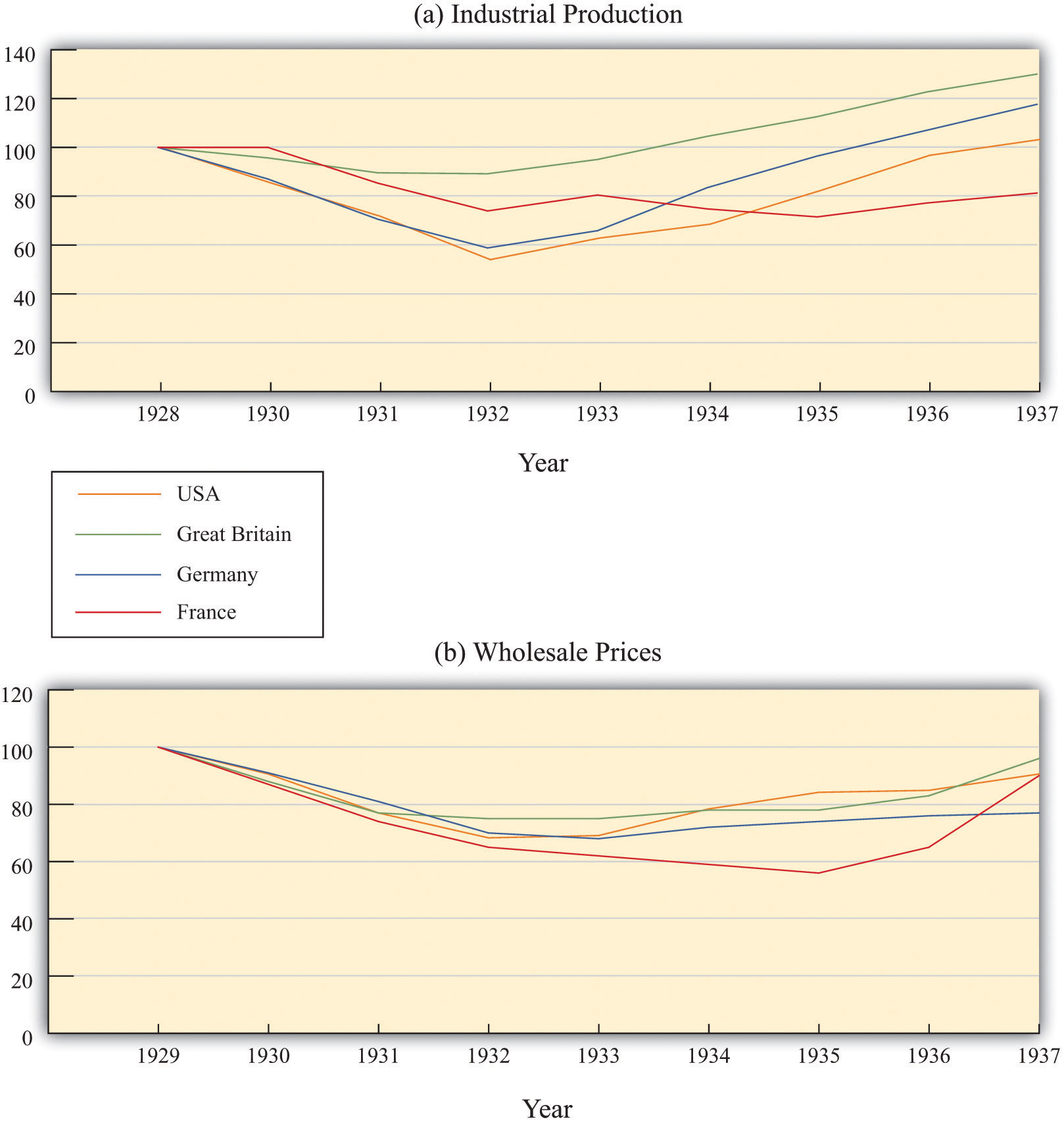
France, Germany, and Britain also experienced declines in output (a) and prices (b) during the Great Depression. The output data are data for industrial production (manufacturing in the case of the United States), and the price data are wholesale prices.
Source: International Monetary Fund, “World Economic Outlook: Crisis and Recovery,” April 2009, Box 3.1.1, http://www.imf.org/external/pubs/ft/weo/2009/01/c3/Box3_1_1.pdf.
Why this was the case remains one of the puzzles of the period. There were events at the time that had international dimensions, such as concerns about the future of the “gold standard” (which determined the exchange rates between countries) and various policies that disrupted international trade. Still, economists are unconvinced that such factors can explain why the Great Depression occurred in so many countries. Three-fourths of a century later, we still do not have a complete understanding of the Great Depression and are still unsure exactly why it happened. From one perspective this is frustrating, but from another it is exciting: the Great Depression maintains an air of mystery.
Toolkit: Section 31.20 "Foreign Exchange Market"
You can review the meaning and definition of the exchange rate in the toolkit.
Try to imagine yourself in the United States or Europe in the early 1930s. You are witnessing immense human misery amid a near meltdown of the economy. Friends and family are losing their jobs and have bleak prospects for new employment. Stores that you had shopped in all your life suddenly go out of business. The bank holding your money has disappeared, taking your savings with it. The government provides no insurance for unemployment, and there is no system of social security to provide support for your elderly relatives.
Economists and government officials at that time were bewildered. The experience in the United States and other countries was difficult to understand. According to the economic theories of the day, it simply was not possible. Policymakers had no idea how to bring about economic recovery. Yet, as you might imagine, there was considerable pressure for the government to do something about the problem. The questions that vexed the policymakers of the day—questions such as “What is happening?” and “What can the government do to help?”—are at the heart of this chapter.
Economists make sense of events like the Great Depression by first accumulating facts and then using frameworks to interpret those facts. We have a considerable advantage relative to economists and politicians at the time. We have the benefit of hindsight: the data we looked at in the previous subsection were not known to the economists of that era. And economic theory has evolved over the last seven decades, giving us better frameworks for analyzing these data.
Earlier, we said there are two possible reasons why output decreased.
We look at each of these candidate explanations in turn.
Toolkit: Section 31.26 "The Aggregate Production Function"
You can review the aggregate production function and the inputs that go into it in the toolkit.
After you have read this section, you should be able to answer the following questions:
Our first approach to interpreting the Great Depression focuses on potential outputThe amount of real GDP the economy produces when the labor market is in equilibrium and capital goods are not lying idle., which is the amount of real gross domestic product (real GDP) an economy produces when the labor market is in equilibrium and capital goods are not lying idle. We start here because this approach corresponds reasonably closely to the economic wisdom of the time.
Comparative statics is a technique that allows us to understand the effects of a decrease in technology in a particular market, such as the market for new homes. In a comparative statics exercise, we look at what happens to endogenous variables (in this case, production and prices of new homes) when we change an exogenous variable (in this case, technology). A decline in technology shifts the market supply curve leftward: at any given price, the decrease in technology means that the firm can produce less output with its available inputs. The result is shown in part (a) of Figure 22.4 "An Inward Shift in the Market Supply of Houses" for the housing market: output of new homes decreases and the price of new homes increases.
Toolkit: Section 31.16 "Comparative Statics"
You can review the technique of comparative statics and the definition of endogenous and exogenous variables in the toolkit.
Figure 22.4 An Inward Shift in the Market Supply of Houses
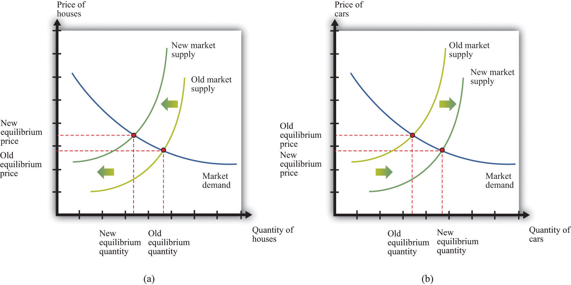
(a) A decrease in technology leads to an inward shift of the market supply curve for houses. (b) The labor and other resources that are not being used to produce houses can now be used to produce other goods, such as cars.
If this decline in technology in the housing market were the only change in the economy, what would happen? Construction firms would fire workers because these firms were building fewer new homes. Over time, however, the fired construction workers would find new jobs in other sectors of the economy. The same logic applies to other inputs: capital and other inputs that were being used in the construction industry would be redeployed to other markets. For example, there would be additional labor and other inputs available for automobile production. Part (b) of Figure 22.4 "An Inward Shift in the Market Supply of Houses" shows the resulting outward shift in the supply curve for cars. It is difficult to explain the big decrease in output and the high rate of unemployment in the Great Depression through a change in technology in a single market.
Suppose, however, that this change in technology does not happen in just one market but occurs across the entire economy. Then a version of part (a) in Figure 22.4 "An Inward Shift in the Market Supply of Houses" would hold for each market in the economy. We would see declines in economic activity across a wide range of markets. Moreover, with declines in so many industries, we would expect to see lower real wages and less employment. The idea that workers could easily move from one industry to another is not as persuasive if the entire economy is hit by an adverse technology shock.
We use growth accounting to show how changes in output are driven by changes in the underlying inputs—capital, labor, and technology. Equivalently, we use the technique to give us a measure of the growth rate of technology, given data on the growth rates of output, capital, and labor:
technology growth rate = output growth rate − [a × capital stock growth rate] − [(1 − a) × labor growth rate].We have omitted human capital from this growth accounting equation. We do so because, unfortunately, we do not have very good human capital measures for the period of the Great Depression. Human capital typically changes very slowly, so this is not too much of a problem: over a period of a decade, we do not expect big changes in human capital. Any changes in human capital that do occur are included in the catchall “technology” term.
Toolkit: Section 31.28 "Growth Accounting"
You can review the technique of growth accounting in the toolkit.
The key ingredient needed for the growth accounting equation is the number a. It turns out that a good measure of a is the fraction of real GDP that is paid to owners of capital. Roughly speaking, it is the amount of GDP that goes to the profits of firms. Equivalently, (1 − a) is the fraction of GDP that is paid to labor. The circular flow of income reminds us that all income ultimately finds its way back to households in the economy, which is why these two numbers sum to one.
The economist John Kendrick applied such growth accounting to data from the Great Depression.See John W. Kendrick, Productivity Trends in the United States (Princeton, NJ: Princeton University Press, 1961), particularly Table A-XXII, p. 335, and the discussion of these calculations. Table 22.2 "Growth Rates of Real GDP, Labor, Capital, and Technology, 1920–39*" summarizes his findings. Each row in Table 22.2 "Growth Rates of Real GDP, Labor, Capital, and Technology, 1920–39*" decomposes output growth into three components. In 1923, for example, output grew at a very high rate of 14.2 percent. This growth in output came from labor growth of 9.9 percent and capital stock growth of 2.0 percent. The remainder, which we interpret as growth in technology, grew at 9.5 percent. By all accounts, 1923 was a good year. The other entries in the table can be read in the same way.
Table 22.2 Growth Rates of Real GDP, Labor, Capital, and Technology, 1920–39*
| Year | Real GDP | Labor | Capital | Technology |
|---|---|---|---|---|
| 1920 | 0.4 | 1.4 | 2.1 | −1.2 |
| 1921 | −3.6 | −11.5 | 1.5 | 4.0 |
| 1922 | 6.4 | 8.7 | 0.7 | 0.1 |
| 1923 | 14.2 | 9.9 | 2.0 | 9.5 |
| 1924 | 2.0 | −3.2 | 2.6 | 4.9 |
| 1925 | 3.6 | 4.0 | 2.4 | 0.1 |
| 1926 | 6.2 | 4.2 | 3.2 | 3.4 |
| 1927 | 1.1 | −0.2 | 2.9 | 0.5 |
| 1928 | 1.0 | 0.6 | 2.4 | −0.3 |
| 1929 | 6.5 | 2.2 | 2.4 | 5.7 |
| 1930 | −9.2 | −8.1 | 2.0 | −4.8 |
| 1931 | −7.5 | −10.5 | 0.1 | 0.4 |
| 1932 | −14.5 | −13.5 | −2.2 | −5.2 |
| 1933 | −2.5 | −1.0 | −3.4 | −1.2 |
| 1934 | 9.9 | 0.4 | −2.8 | 13.7 |
| 1935 | 9.0 | 5.8 | −1.4 | 6.6 |
| 1936 | 12.8 | 10.3 | 0.0 | 6.8 |
| 1937 | 6.9 | 5.8 | 1.4 | 2.9 |
| 1938 | −5.5 | −9.3 | 0.9 | 1.2 |
| 1939 | 9.1 | 6.2 | −0.3 | 4.6 |
| *All entries are annual growth rates calculated using data from John W. Kendrick, Productivity Trends in the United States (Princeton, NJ: Princeton University Press, 1961), Table A-XXII, 335. Following the discussion in Kendrick, the capital share (a) was 0.30 until 1928 and 0.25 thereafter. | ||||
Real GDP and technology were both growing in most years in the 1920s. In the early 1930s both variables decreased, and both grew again as the economy recovered from the Great Depression. In other words, technology growth and output growth are positively correlated over this period. This suggests the possibility that changes in technology caused the changes in output—always remembering that, as we observed earlier, correlation need not imply a causal relationship. An improvement in technology causes firms to want to produce more. They demand more workers, so employment and real wages increase. The increased output, through the circular flow, means that there is increased income. Households increase both consumption and savings. Higher savings means higher investment, so, over time, the economy accumulates more capital. Exactly the opposite holds if there is a decrease in technology: in this case, employment, consumption, and investment all decrease.
Does this theory fit the facts? For the roaring twenties, we see growth in output, labor, and capital. In addition, there was a positive technology growth rate in almost all the years of the decade. These movements are indeed consistent with the behavior of an economy driven by improvements in technology. Jumping back for a moment to individual markets, improvements in technology shift supply curves rightward. Increased output is therefore accompanied by decreased prices. The aggregate price level is nothing more than a weighted average of individual prices, so price decreases in individual markets translate into a decrease in the overall price level. From Table 22.1 "Major Macroeconomic Variables, 1920–39*", the price level actually moved very little between 1922 and 1929, so this fits less well.
Overall, the view that technological progress fueled the growth from 1922 to 1929 seems broadly consistent with the facts. Given the simplicity of the framework that we are using, “broadly consistent” is probably the best it is reasonable to hope for.
Now let us apply the same logic to the period of the Great Depression. Negative growth in output from 1930 to 1933 was matched by negative growth in labor and technology (except for 1931). The capital stock decreased from 1932 to 1935, reflecting meager investment during this period. When the economy turned around in 1934, technology growth turned up as well.
Imagine that the economy experienced negative technology growth from 1929 to 1933. The reduced productivity of firms leads to a decrease in demand for labor, so real wages and employment decrease. Lower productivity also means that firms did not think it was worthwhile to invest in building new factories and buying new machinery. Both labor and capital inputs into the production function declined. Once technology growth resumed in 1934, the story was reversed: labor and capital inputs increased, and the economy began to grow again. In this view, there was a substantial decline in the production capabilities of the economy, leading to negative growth in output, consumption, and investment. The Great Depression, in this account, was driven by technological regress.
Many economists are skeptical of such an explanation of the Great Depression. They have three criticisms. First, large-scale technological regress is difficult to believe on its face. Did people know an efficient way to manufacture something in 1929 but then forget it in 1930? Even remembering that technology includes social infrastructure, it is hard to imagine any event that would cause a decrease of 3 percent or more in technology—and if such an event did occur, surely we would be able to point to it and identify it.
Second, this explanation claims that labor input decreased because households saw lower real wages and voluntarily chose to consume leisure rather than work. By most measures, though, real wages increased. Moreover, it is difficult to equate a 25 percent unemployment rate, not to mention all the stories of how people could not find work, with a labor market in which households are simply moving along a labor supply curve.
Third, a prominent feature of the Great Depression is the decrease in the price level that occurred from 1929 to 1933. Table 22.1 "Major Macroeconomic Variables, 1920–39*" tells us that prices decreased by over 9 percent in both 1931 and 1932. However, a reduction in the level of potential GDP would cause an inward shift of market supply curves and thus an increase, rather than a decrease, in prices.
For most economists, the view of the Great Depression as a shift in technology is not convincing. Something else must have been going on. In particular, the very high unemployment rate strongly suggests that labor markets were malfunctioning. Thus, rather than viewing the large decreases in output in economies around the world as part of the normal functioning of supply and demand in an economy, we should perhaps consider it as evidence that sometimes things can go badly wrong with the economy’s self-correction mechanisms. If we want to explain the Great Depression, we are then obliged—as were the economists at the time—to find a new way of thinking about the economy. It was an economist named John Maynard Keynes who provided such a new approach; in so doing, he gave his name to an entire branch of macroeconomic theory.
After you have read this section, you should be able to answer the following questions:
In his analysis of the Great Depression, John Maynard Keynes contrasted his new approach with the prevailing “classical” theory:John Maynard Keynes, The General Theory of Employment, Interest and Money (Orlando: First Harvest/Harcourt, 1964[1936]), 3. “I shall argue that the postulates of the classical theory are applicable to a special case only and not to the general case.…Moreover, the characteristics of the special case assumed by the classical theory happen not to be those of the economic society in which we actually live, with the result that its teaching is misleading and disastrous if we attempt to apply it to the facts of experience.” Keynes claimed that there was a fundamental failure in the economic system that prevented markets from fully coordinating activities in the economy. He argued that, as a consequence, the actual output of the economy was not determined by the productive capacity of the economy, and that it was “misleading and disastrous” to think otherwise. In more modern terms, he said that actual output need not always equal potential output but was instead determined by the overall level of spending or demand in the economy.
Keynes provided a competing story of the Great Depression that did not rely on technological regress and in which unemployment truly reflected an inability of households to find work. Keynes gave life to aggregate spendingThe total amount of spending by households, firms, and the government on the goods and services that go into real GDP.—the total spending by households, firms, and governments—as a determinant of aggregate gross domestic product (GDP). With this new perspective, Keynes also uncovered a way in which government intervention might help the functioning of the economy.
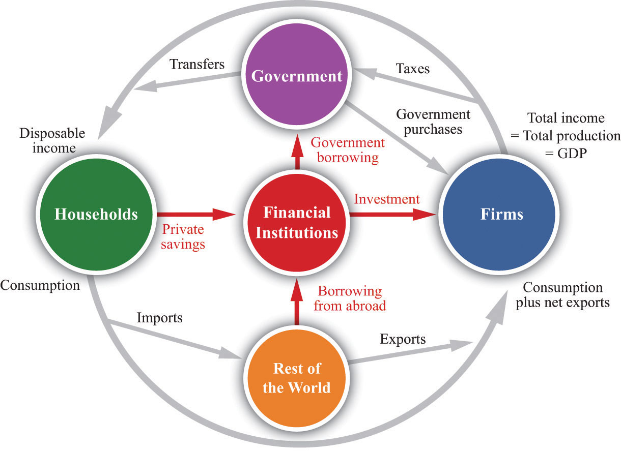
To understand how Keynes approached the puzzle of the Great Depression, we must first look more closely at the components of GDP. Figure 22.5 "The Firm Sector in the Circular Flow" shows the circular flow, emphasizing the flows in and out of the firm sector of the economy. Accounting rules tell us that in every sector of the circular flow, the flow of dollars in must equal the flow of dollars out. We know that the total flow of dollars from the firm sector measures the total value of production in the economy. The total flow of dollars into the firm sector equals total expenditures on GDP. The figure therefore illustrates a fundamental relationship in the national accounts.
Figure 22.5 The Firm Sector in the Circular Flow
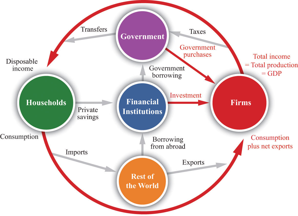
The flow of dollars into the firm sector equals consumption plus net exports plus investment plus government purchases. The flow of dollars from the firm sector equals total GDP in the economy.
The national income identityProduction equals the sum of consumption plus investment plus government purchases plus net exports. states that
production = consumption + investment + government purchases + net exports.Toolkit: Section 31.27 "The Circular Flow of Income"
The toolkit describes the circular flow of income in more detail.
ConsumptionThe total spending by households on final goods and services. refers to total consumption spending by households on final goods and services. Consumption is divided into three categories.
The distinctions among these categories are not always as clear-cut as the definitions suggest. A good pair of blue jeans might outlast a shoddy dishwasher, even though the jeans are classified as a nondurable good and the dishwasher as a durable good.
InvestmentThe purchase of new goods that increase capital stock, allowing an economy to produce more output in the future. is the purchase of new goods that increase the capital stock, allowing us to produce more output in the future. Investment is divided into three categories.
The economist’s definition of investment is precise and differs from the way we often use the word in everyday speech. Specifically, economists do not use the term to mean the purchase of financial assets, such as stocks and bonds. Most of the time when we talk about investment in this book, we are referring to business fixed investment—the production of new physical capital goods. Inventory investment is a special category of investment that we explain in Section 22.3.2 "Inventory Investment".
As a rough rule of thumb, consumption spending is carried out by households, and investment spending is carried out by firms. But there is one important exception: new residential construction is included in investment. A new house purchased by a household is treated as investment, not consumption.
Government purchasesSpending by the government on goods and services. include all purchases of goods and services by the government. We include in our definition of “government” local as well as national government activity. In the United States, this means that we collapse together federal, state, and local governments for the purpose of our analysis.
This component of spending refers only to purchases of goods and services, not to transfersA cash payment from the government to individuals and firms.. So, if the federal government buys aircraft from Boeing or the local police department buys a fleet of Volvos, these are included in government purchases. However, a transfer you receive from the government—say, because you are unemployed and are being paid unemployment insurance—is not counted in GDP. (Of course, if you then use this income to purchase goods and services, that consumption is part of GDP.)
Net exportsExports minus imports. simply equal exports minus imports. They are included because we must correct for the expenditure flows associated with the rest of the world. Some spending in the economy goes to imported goods, which is not associated with domestic production. We must subtract these imports from total expenditures. Against that, some demand for domestically produced goods comes from other countries. We add these exports to total expenditure.
Inventory investment is a relatively minor component of GDP, but we need to understand it in some detail because it plays a key role in the Keynesian approach. When a firm produces output, it does one of two things with it: it either sells it or adds it to inventory. Thus an accounting relationship within a firm is that
production = sales + changes in inventory.If a firm produces more than it sells, its stocks of inventories increase. If a firm sells more than it produces, its stocks of inventories decrease. The inventories that a firm holds are counted as part of its capital stock, so any change in firms’ inventories is counted as a component of investment.
Suppose General Motors (GM) produces 10 million cars, anticipating that it will sell them all. Then imagine that demand is lower than expected, so it only sells 9.9 million. The result is that 100,000 cars pile up on GM’s lots, and the GM accountants record this as an addition to inventory. We want GDP to measure both production and spending, but we have 100,000 cars that have been produced but not purchased. The national income accounts get around this problem by effectively pretending that GM bought the cars from itself.
If the cars are then sold in the following year, they will not contribute to GDP in that year—quite properly, since they were not produced that year. The national accounts in the next year will show that 100,000 cars were sold to households, but they will also show that inventories decreased by 100,000 cars. Thus the accounts record expenditures on these cars as part of durable goods consumption, but the accounts also contain an offsetting reduction in inventory investment.
In some cases, firms change their stocks of inventory as a part of their business strategy. More often, changes in inventories occur because a firm did not correctly forecast its sales. Unplanned inventory investmentAn increase in inventories that comes about because firms have sold less than they anticipated. is an increase in inventories that comes about because a firm sells less than it anticipated. Because GM expected to sell all 10 million cars but sold only 9.9 million, GM had 100,000 cars of unplanned inventory investment.
Moreover, GM is likely to react swiftly to this imbalance between its production plans and its sales. When it sees its sales decrease and its inventory increase, it will respond by cutting its production back until it is in line with sales again. Thus, when an individual firm sees inventories increase and sales decrease, it typically scales down production to match the decrease in demand.
Now let us think about how this works at the level of an economy as a whole. Suppose we divide total spending in the economy into unplanned inventory investment and everything else, which we call planned spendingAll expenditures in an economy except for unplanned inventory investment..
Toolkit: Section 31.30 "The Aggregate Expenditure Model"
Planned spending is all expenditure in the economy except for unplanned inventory investment:
GDP = planned spending + unplanned inventory investment.This equation must always hold true because of the rules of national income accounting.
Begin with the situation where there is no unplanned inventory investment—so GDP equals planned spending—and then suppose that planned spending decreases. Firms find that their production is in excess of their sales, so their inventory builds up. As we just argued, they respond by decreasing production so that GDP is again equal to planned spending, and unplanned inventory investment is once again zero. Thus, even though unplanned inventory investment can be nonzero for very short periods of time, we do not expect such a situation to persist. We expect instead that actual output will, in fact, almost always equal planned spending.
Now let us look at how these components of GDP behaved during the 1930s. Table 22.3 "Growth Rates of Key Macroeconomic Variables, 1930–39*" presents these data in the form of growth rates. Remember that a positive growth rate means the variable in question increased from one year to the next, while a negative growth rate means it decreased.
Table 22.3 Growth Rates of Key Macroeconomic Variables, 1930–39*
| Growth Rates | 1930 | 1931 | 1932 | 1933 | 1934 | 1935 | 1936 | 1937 | 1938 | 1939 |
|---|---|---|---|---|---|---|---|---|---|---|
| Real GDP | −8.6 | −6.4 | −13.0 | −1.3 | 10.8 | 8.9 | 13.0 | 5.1 | −3.4 | 8.1 |
| Consumption | −5.3 | −3.1 | −8.9 | −2.2 | 7.1 | 6.1 | 10.1 | 3.7 | −1.6 | 5.6 |
| Investment | −33.3 | −37.2 | −69.8 | 47.5 | 80.5 | 85.1 | 28.2 | 24.9 | −33.9 | 28.6 |
| Government Purchases | 10.2 | 4.2 | −3.3 | −3.5 | 12.8 | 2.7 | 16.7 | −4.2 | 7.7 | 8.8 |
| *This table shows growth rates in real GDP, consumption, investment, and government purchases. All data are from the National Income and Product Accounts web page, Bureau of Economic Analysis, Department of Commerce (http://www.bea.gov/national/nipaweb/index.asp). | ||||||||||
We see again that real GDP decreased for four years in succession (the growth rates are negative from 1930 to 1933). The decrease in real GDP was accompanied by a decline in consumption and investment: consumption likewise decreased for four successive years, and investment decreased for three successive years. The decline in consumption was not as steep as the decline in real GDP, while the decline in investment was much larger. Were we to drill deeper and look at the components of consumption, we would discover that expenditures on durable goods decreased by 17.6 percent in 1930 and 25.1 percent in 1932, while expenditures on services decreased by only 2.5 percent in 1930 and 6.3 percent in 1932.
Whatever was happening during this period evidently had a much larger influence on firms’ purchases of investment goods, and on households’ spending on cars and other durable goods, than it did on purchases of nondurable goods (such as food) and services (such as haircuts). A similar pattern can be observed in modern economies: consumption is smoother than output, and spending on services is smoother than spending on durables. The reason for this is a phenomenon that economists call consumption smoothingThe idea that households like to keep their flow of consumption relatively steady over time, smoothing over income changes..
Toolkit: Section 31.34 "The Life-Cycle Model of Consumption"
Consumption smoothing is the idea that households like to keep their flow of consumption relatively steady over time. When income is unusually high, the household saves (or pays off existing loans); when income is unusually low, the household borrows (or draws down existing savings). Consumption smoothing is a key ingredient of the life-cycle model of consumption, which is discussed in more detail in the toolkit.
If your company has a good year and you get a big bonus, you will increase consumption spending not only this year but also in future years. To do so, you must save a portion of your bonus to pay for this higher consumption in the future. By the same logic, if your income decreases, your consumption will not decrease as much. People who became unemployed during the Great Depression did not reduce their consumption of services and nondurable goods to zero. Instead, as far as was possible, they drew on their existing savings, borrowed, and postponed purchases of durable goods.
Consumption of durable goods, in other words, resembles investment rather than consumption of nondurable goods and services. This makes sense because durable goods resemble investment goods that are purchased by households. Like investment goods, they yield benefits over some prolonged period of time. As an example, consider automobile purchases during the Great Depression. Although 5.4 million cars were produced in 1929, only 3.4 million were produced in 1930—a reduction of more than 37 percent in a single year. Instead of buying new cars, households simply held onto their existing cars longer. As a consequence of the boom of the 1920s, there were a lot of relatively new cars on the road in 1929: the number of cars less than 3 years old was about 9.5 million. Two years later, this number had fallen to 7.9 million.These figures are from Michael Bernstein, The Great Depression: Delayed Recovery and Economic Change in America, 1929–39 (Cambridge, MA: Cambridge University Press, 1987).
This reduction in activity in the automobile industry was matched by a reduction of inputs into the production process. By early 1933, there were only 4 workers for every 10 who had been employed 4 years previously. Equipment purchases for the transportation sector were so low that capital stock for this sector decreased between 1931 and 1935. In the turmoil of the Great Depression, many small car producers went out of business, leaving a few relatively large companies—such as Ford Motor Company and GM—still in business.
Similar patterns arose as the economy recovered. Investment, in particular, was astonishingly volatile. It decreased by about one-third in 1930 and again in 1931, and by over two-thirds in 1932, but rebounded at an astoundingly high rate after 1933. Consumption, meanwhile, grew at a slower rate than GDP as the economy recovered.
After you have read this section, you should be able to answer the following questions:
Now that we understand the components of aggregate spending, we can consider whether a decrease in one or more of these components can explain the Great Depression.
Consider, as before, the market for new houses and suppose there is a reduction in spending on houses. Market demand shifts inward, causing a decrease in the price of houses, as shown in Figure 22.6 "An Inward Shift in Market Demand for Houses". The lower price means that construction firms choose to build fewer houses; there is a movement along the supply curve.
Figure 22.6 An Inward Shift in Market Demand for Houses
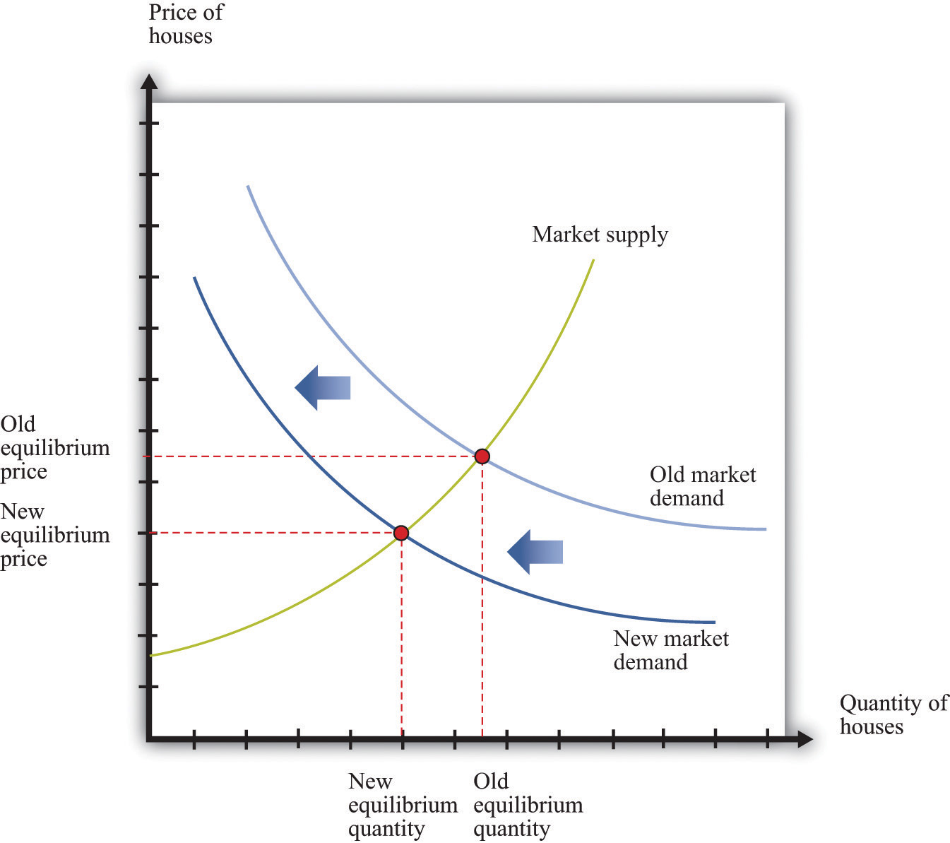
A decrease in demand for houses leads to a decrease in the price of houses and a lower quantity of houses being produced and sold.
As before, the effects are not confined to the housing market. Construction firms demand less labor, so the wages of these workers decrease. Employment in the construction industry declines, but these workers now seek jobs in other sectors of the economy. The increased supply of labor in these sectors reduces wages and thus makes it more attractive for firms to increase their hiring. Supply curves in other sectors shift rightward. Moreover, the income that was being spent on housing will instead be spent somewhere else in the economy, so we expect to see rightward shifts in demand curves in other sectors as well. In summary, if we are looking at the whole economy, a decrease in spending in one market is not that different from a decrease in technology in one market: we expect a reduction in one sector to lead to expansions in other sectors. The economy still appears to be self-stabilizing.
In this story, as is usual when we use supply and demand, we presumed that prices and wages adjust quickly to bring supply and demand into line. This is critical for the effective functioning of markets: for markets to do a good job of matching up demand and supply, wages and prices must respond rapidly to differences between supply and demand. Flexible pricesPrices that adjust immediately to shifts in supply and demand curves so that markets are always in equilibrium. adjust immediately to shifts in supply and demand curves so that price is always at the point where supply equals demand. If, for example, the quantity of labor supplied exceeds the quantity of labor demanded, flexible wages decrease quickly to bring the labor market back into equilibrium.
Suppose we instead entertain the possibility that wages and prices do not immediately adjust. Sticky pricesPrices that do not adjust immediately to shifts in supply and demand curves so that markets are not always in equilibrium. do not react immediately to shifts in supply and demand curves, and the adjustment to equilibrium can take some time. We defer for the moment the discussion of why prices might be sticky and concentrate instead on the implications of this new idea about how markets work. The easiest way to see the effects of price stickiness is to suppose that prices do not change at all. Figure 22.7 "A Shift in Demand for Houses When Prices Are Sticky" shows the impact of a decrease in demand for houses when the price of houses is completely sticky. If you compare Figure 22.7 "A Shift in Demand for Houses When Prices Are Sticky" to Figure 22.6 "An Inward Shift in Market Demand for Houses", you see that a given shift in demand leads to a larger change in the quantity produced.
Figure 22.7 A Shift in Demand for Houses When Prices Are Sticky
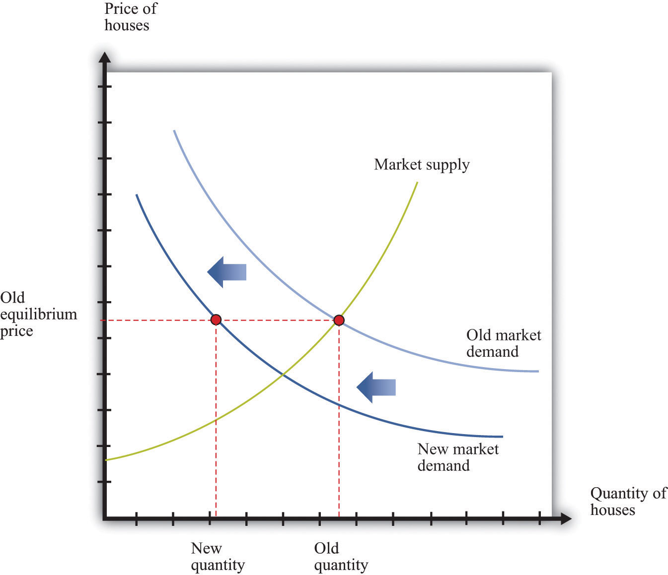
If the price in the market is “sticky,” it may not adjust immediately to the change in demand, resulting in a large decrease in the quantity of houses that are produced and sold.
What about the effects on other markets? As before, a decrease in demand for housing will cause construction workers to lose their jobs. If wages are sticky, these workers may become unemployed for a significant period of time. Their income decreases, and they consume fewer goods and services. So, for example, the demand for beef in the economy might decrease because unemployed construction workers buy cheaper meat. This means that the demand for beef shifts inward. The reduction in activity in the construction sector leads to a reduction in activity in the beef sector. And the process does not stop there—the reduced income of cattle farmers and slaughterhouse workers will, in turn, spill over to other sectors.
What has happened to the self-stabilizing economy described earlier? First, sticky wages and prices impede the incentives for workers to flow from one sector to another. If wages are sticky, then the reduction in labor demand in the construction sector does not translate into lower wages. Thus there is no incentive for other sectors to expand. Instead, these other sectors, such as food, see a decrease in demand for their product, which leads them to contract as well. Second, the decrease in income means that it is possible to see decreases in demand across the entire economy. It no longer need be the case that reductions in spending in one area lead to increased spending in other sectors.
So far, we have told this story in terms of individual markets. The circular flow helps us see how these markets come together in the aggregate economy. When we looked at the markets for housing and beef, we saw that a decrease in demand for housing led to a decrease in demand for labor and, hence, to lower labor income. We also saw that as income earned in the housing market decreased, spending decreased in the beef market. Such linkages are at the heart of the circular flow of income. Household spending on goods and services is made possible by a flow of income from firms. Firms’ hiring of labor is made possible by a flow of revenue from households. Keynes argued that this was a delicate process that might be prone to malfunction in a variety of ways.
Households are willing to buy goods and services if they have a reasonable expectation that they can earn income by selling labor. During the Great Depression, however, household expectations were surely quite pessimistic. Individuals without jobs believed that their chances of finding new employment were low. Those lucky enough to be employed knew that they might soon be out of work. Thus households believed it was possible, even likely, that they would receive low levels of income in the future. In response, they cut back their spending.
Meanwhile, the willingness of firms to hire labor depends on their expectation that they can sell the goods they manufacture. When firms anticipate a low level of demand for their products, they do not want to produce much, so they do not need many workers. Current employees are laid off, and there are few new hires.
Through the circular flow, the pessimism of households and the pessimism of firms interact. Firms do not hire workers, so household income is low, and households are right not to spend much. Households do not spend, so demand for goods and services is low, and firms are right not to hire many workers. The pessimistic beliefs of firms and workers become self-fulfilling prophecies.
In the remainder of this section, we build a framework around the ideas that we have just put forward. The framework focuses on the determinants of aggregate spending because, in this approach, the output of the economy is determined not by the level of potential output but by the level of total spending. This model is based around the idea of sticky prices—or, more precisely, it tells us what the output of the economy will be, at a given value of the overall price level. Once we understand this, we can add in the effects of changing prices.
Earlier, we introduced the national income identity:
production = consumption + investment + government purchases + net exports.This equation must be true by the way the national income accounts are constructed. That is, it is an accounting identity. We also explained that
GDP = planned spending + unplanned inventory investment.It is possible for firms to accumulate or decumulate inventories unintentionally, but such a situation will not persist for long. Firms quickly respond to such imbalances by adjusting their production. The aggregate expenditure model takes the national income identity and adds to it the condition that unplanned inventory investment equals zero—equivalently, gross domestic product (GDP) equals planned spending:
planned spending = consumption + investment + government purchases + net exports.Another way of saying this is that as long as we interpret investment to include only planned investment, the national income equation is no longer an identity but instead a condition for equilibrium.
We could now examine all four components of planned spending separately.Different chapters of this book delve deeper into these types of spending. For the moment, however, we group them all together. We focus on the fact that total planned spending depends positively on the level of income and output in an economy, for two main reasons:
Figure 22.8 The Planned Spending Line
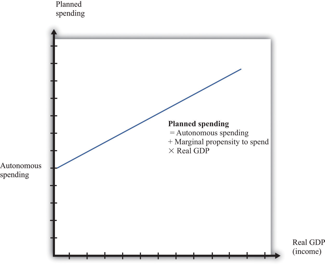
Planned spending is composed of autonomous spending (the amount of spending when real GDP equals zero) and induced spending (spending resulting from real GDP).
In summary, we conclude that when income increases, planned expenditure also increases. We illustrate this in Figure 22.8 "The Planned Spending Line", where we suppose for simplicity that the relationship between planned spending and GDP is a straight line:
planned spending = autonomous spending + marginal propensity to spend × GDP.Autonomous spendingThe amount of spending that there would be in an economy if income were zero. is the intercept of the planned spending line. It is the amount of spending that there would be in an economy if income were zero. It is positive, for two reasons: (1) A household with no income still wants to consume something, so it will either draw on its existing savings or borrow against future income. (2) The government purchases goods and services even if income is zero.
The marginal propensity to spendThe slope of the planned spending line, measuring the change in planned spending if income increases by $1. is the slope of the planned spending line. It tells us how much planned spending increases if there is a $1 increase in income. The marginal propensity to spend is positive: Increases in income lead to increased spending by households and firms. The marginal propensity to spend is less than one, largely because of consumption smoothing by households. If household income increases by $1, households typically consume only a fraction of the increase, saving the remainder to finance future consumption. This equation, together with the condition that GDP equals planned spending, gives us the aggregate expenditure modelThe framework that links planned spending and output..
Toolkit: Section 31.30 "The Aggregate Expenditure Model"
The aggregate expenditure model takes as its starting point the fact that GDP measures both total spending and total production. The model focuses on the relationships between output and spending, which we write as follows:
planned spending = GDP and planned spending = autonomous spending + marginal propensity to spend × GDP.The model finds the value of output for a given value of the price level. It is then combined with a model of price adjustment to give a complete picture of the economy.
Figure 22.9 Equilibrium in the Aggregate Expenditure Model
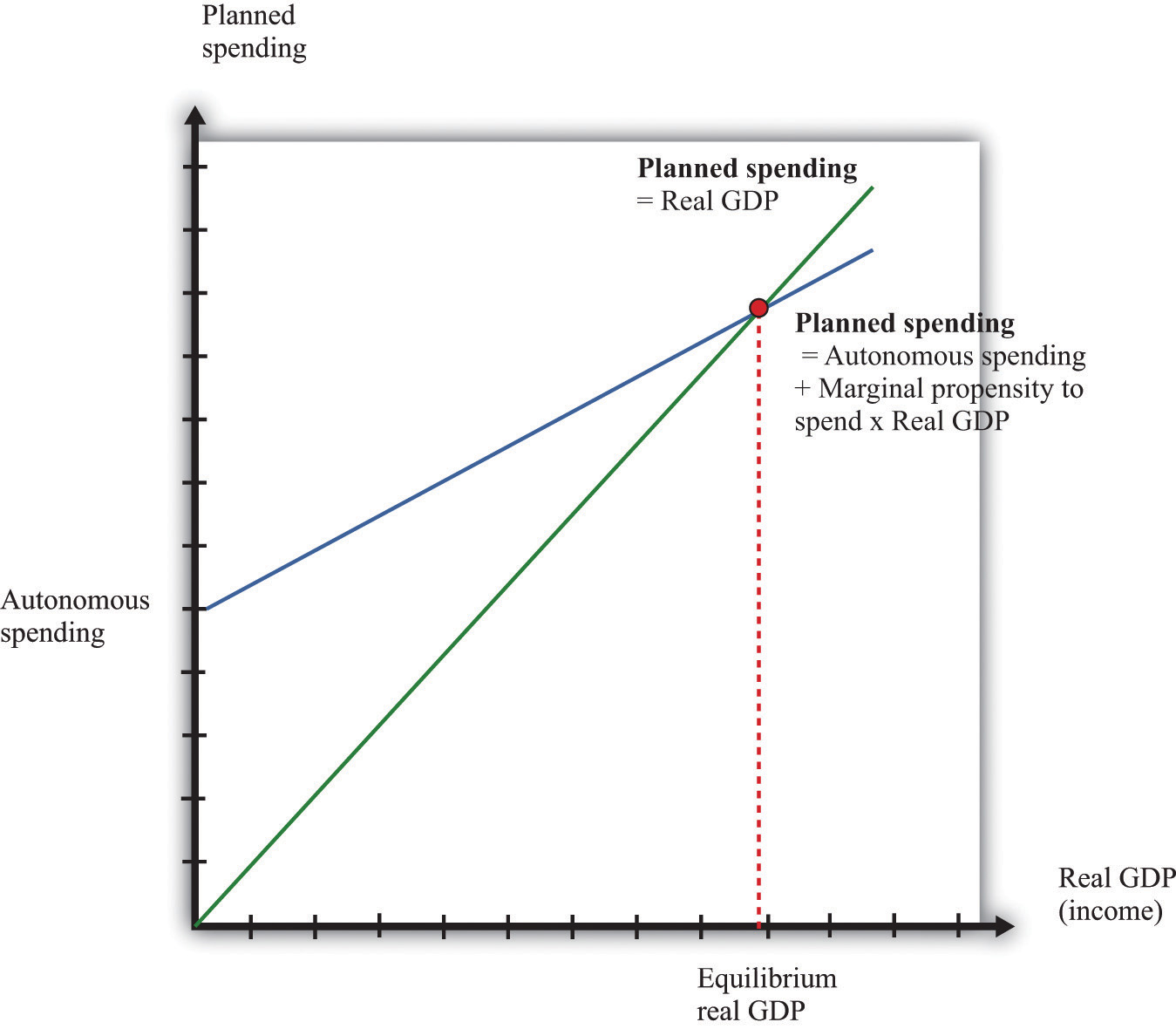
The aggregate expenditure framework tells us that the economy is in equilibrium when planned spending equals real GDP.
We can solve the two equations to find the values of GDP and planned spending that are consistent with both equations:
We can also take a graphical approach, as shown in Figure 22.9 "Equilibrium in the Aggregate Expenditure Model". On the horizontal axis is the level of real GDP, while on the vertical axis is the overall level of (planned) spending in the economy. We graph the two relationships of the aggregate expenditure model. The first line is a 45° line—that is, it is a line with a slope equal to one and passing through the origin. The second is the planned spending line. The point that solves the two equations is the point where the two lines intersect. This diagram is the essence of the aggregate expenditure model of the macroeconomy.
The aggregate expenditure model makes no reference to potential output or the supply side of the economy. The model assumes that the total amount of output produced will always equal the quantity demanded at the given price. You might think that this neglect of the supply side is a weakness of the model, and you would be right. In Section 22.4.6 "Price Adjustment", when we introduce the adjustment of prices, the significance of potential output becomes clear.
We now apply this framework to the Great Depression. The aggregate expenditure approach suggests that output decreased in the Great Depression because aggregate spending decreased. Part (a) of Figure 22.10 "A Decrease in Aggregate Expenditures" shows how this process begins: a decrease in autonomous spending shifts the spending line down. The interpretation of such a shift is that, at every level of income, spending is lower. Such a decrease in spending is due to a decrease in (the autonomous component of) consumption, investment, government spending, or net exports (or some combination of these). Part (b) of Figure 22.10 "A Decrease in Aggregate Expenditures" shows what happens when the planned spending line shifts downward. The equilibrium level of real GDP decreases. So far, therefore, the aggregate expenditure model seems to work: a decrease in autonomous spending leads to a decrease in real GDP at the given price level. But we need to know why planned spending decreased.
Figure 22.10 A Decrease in Aggregate Expenditures
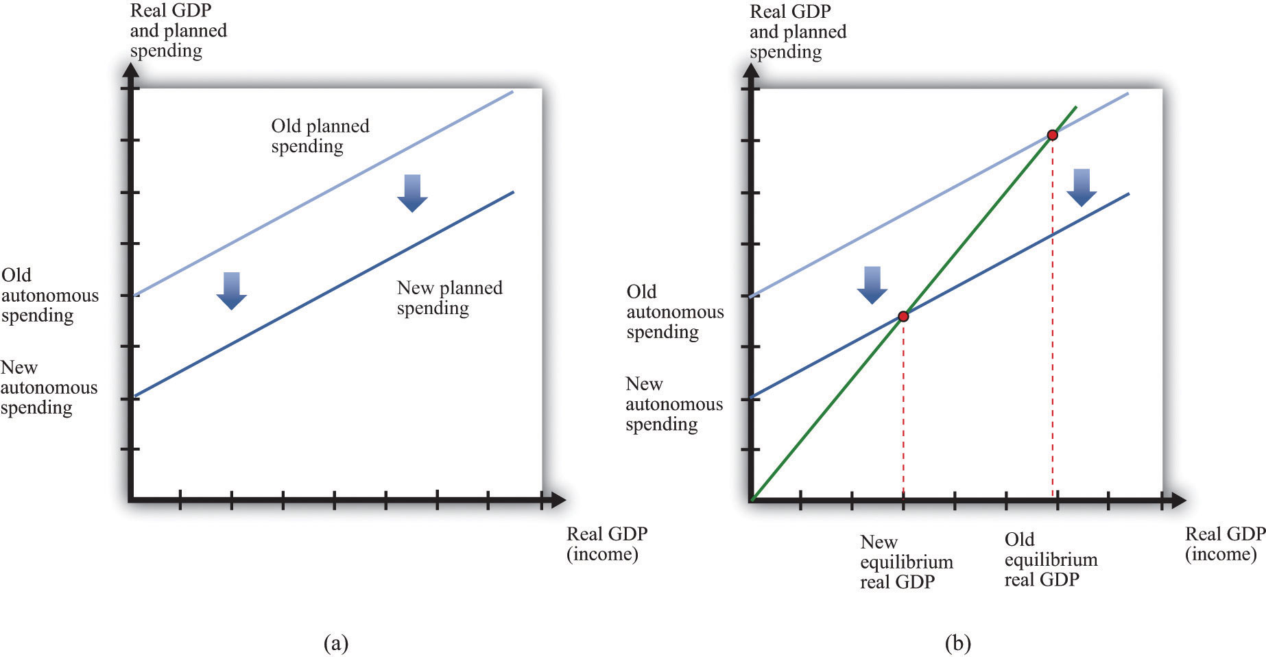
The Keynesian explanation of the Great Depression is that a decrease in autonomous spending caused the planned spending line to shift downward (a) leading to a decrease in the equilibrium level of real GDP (b).
Let us first consider the possibility that a reduction in consumption triggered the Great Depression. Recall that, between September and November 1929, the stock market in the United States crashed. This collapse meant that many households were suddenly less wealthy than they had been previously. A natural response to a decrease in wealth is to decrease consumption; this is known as a wealth effectThe effect on consumption of a change in wealth..
Wealth is distinct from income. Income is a flow: a household’s income is the amount that it receives over a period of time, such as a year. Wealth is a stock: it is the cumulated amount of the household’s savings. Is it plausible that wealth effects could explain a collapse of the magnitude of the Great Depression? To answer this, we need to determine how much real GDP decreases for a given change in autonomous spending.
Toolkit: Section 31.30 "The Aggregate Expenditure Model"
The solution for output in the aggregate expenditure model can be written in terms of changes as follows:
change in GDP = multiplier × change in autonomous spending,where the multiplierThe amount by which a change in autonomous spending must be multiplied to give the change in output, equal to 1 divided by (1 – the marginal propensity to spend). is given by
Suppose that the marginal propensity to spend is 0.8. Then
A given change in autonomous spending will lead to a fivefold change in real GDP. Economists refer to this as a multiplier process. Because (1 − marginal propensity to spend) is less than one, the multiplier is a number greater than one. This means that any change in autonomous spending is multiplied up to result in a larger change in GDP. Even relatively small decreases in spending can end up being damaging to an economy.
The economics behind the multiplier comes from the circular flow of income. Begin with a decrease in autonomous spending. The reduction in spending means less demand for firms’ goods and services. Firms respond by cutting output. (As a reminder, the signal to firms that they should cut their output comes from the fact that they see a buildup of their inventory.) When firms cut their output, they require less labor and pay out less in wages, so household income decreases. This causes households to again cut back on consumption, so spending decreases further. Thus we go round and round the circular flow diagram: decreased spending leads to decreased output, which leads to decreased income, which leads to decreased spending, which leads to decreased output, and so on and so on. The process continues until the reductions in income, output, and consumption in each round are tiny enough to be ignored.
We use the multiplier to carry out comparative static exercises in the aggregate expenditure model. In this case, the endogenous variable is real GDP, and the exogenous variable is autonomous spending. Given a change in autonomous spending, we simply multiply by the multiplier to get the change in real GDP when the price level is fixed. Let us do some back-of-the-envelope comparative static calculations, based on the assumption that the marginal propensity to spend is 0.8, so the multiplier is 5.
Table 22.1 "Major Macroeconomic Variables, 1920–39*" tells us that real GDP decreased by approximately $75 billion between 1929 and 1930. With a multiplier of 5, we would need a drop in autonomous spending of $75 billion divided by 5, or $15 billion, to get this large a decrease in GDP. The population of the United States in 1930 was approximately 123 million, so a $15 billion decrease in spending corresponds to about $122 per person. Remember that the figures in Table 22.1 "Major Macroeconomic Variables, 1920–39*" are in terms of year 2000 dollars. It certainly seems plausible that households, who had been made significantly poorer by the collapse in the stock market, would have responded by cutting back spending by the equivalent today of a few hundred dollars per year.
Our goal, you will remember, is to explain the events of the Great Depression. How are we doing so far? The good news is that we do have a story that explains how output could decrease as precipitously as it did in the Great Depression years: there was a major stock market crash, which made people feel less wealthy, so they decided to consume less and save more.
If we look more closely, though, this story still falls short. When we examined the data for the Great Depression, we saw that—while output and consumption both decreased—consumption decreased much less than did output. For example, from 1929 to 1933, real GDP decreased by 26.5 percent, while consumption decreased by 18.2 percent. By contrast, investment (that is, purchases of capital by firms, new home construction, and changes in business inventories) decreased much more than output. In 1932, purchases of new capital were $11 billion (year 2000 dollars), compared to a level of $91 billion in 1929. This is a reduction in real investment of about 82 percent. We must look more closely at investment to see if our theory can also explain the different behavior of consumption and investment.
When GDP decreases, there can be an induced decrease in investment: declines in income lead firms to anticipate lower production in the future, meaning they see less of a need to build up their capital stock. But the changes in investment during the Great Depression were very large. Because it is implausible that such large variation was the result of changes in output alone, economists look for additional explanations of why investment decreased so much during the Great Depression.
During the Great Depression, the link between savings and investment was disrupted by bank failures. Between 1929 and 1933, a number of US banks went out of business, often taking the savings of households with them. People began to trust banks less, and many households stopped putting their savings into the financial sector. The financial sector is an intermediary between households and firms, matching up the supply of savings from households with the demand for savings by firms. Figure 22.11 "The Financial Sector in the Circular Flow of Income" shows the flows in and out of the financial sector. (Our focus here is on the role of this sector in matching savers and investors. As Figure 22.11 "The Financial Sector in the Circular Flow of Income" shows, however, funds also flow into (or from) the financial sector from the rest of the world and the government sector.)
Figure 22.11 The Financial Sector in the Circular Flow of Income
Financial institutions such as banks act as intermediaries in the circular flow of income. During the Great Depression, many banks failed, disrupting the matching of savings and investment.
To understand bank failures in the Great Depression, we need to take a moment to review what banks do. A bank is an institution that accepts money (“bank deposits”) from individuals. It then takes some of that money and puts it into longer-term projects—the construction of an apartment building, for example. The bank in this case issues a long-term loan to the company that plans to construct the new building.
At any time, a bank has a portfolio of assets. Some are liquidCapable of being easily and quickly exchanged for cash.; they are easily and quickly exchanged for cash. Some are illiquidNot capable of being easily and quickly exchanged for cash.; they cannot easily be converted into cash. Banks keep some assets in a highly liquid form, such as cash or very short-term loans, and also hold assets that are relatively illiquid, such as a two-year loan to a construction company.
At any time, depositors at a bank can choose to withdraw their money. Under normal circumstances, people are happy to leave most of their money in the bank, so only a small fraction of depositors want to withdraw money on any given day. The bank keeps some cash in its vaults to accommodate this demand. But suppose that times are not normal. Suppose that, as was the case during the Great Depression, depositors start to see that other banks are going out of business. Then they may worry that their own bank is also at risk of failing, in which case they will lose their savings. The natural response is to rush to the bank to withdraw money before the bank fails.
If a large number of depositors all try to withdraw money at once, the bank will run out of cash and other liquid assets. It will not be able to meet the needs of its depositors. The consequence is a bank runA significant fraction of a bank’s depositors all trying to withdraw funds at the same time.. And if the bank is unable to meet its depositors’ demands, it may be forced out of business altogether. This is known as a bank failureWhen a bank closes because it is unable to meet its depositors’ demands..
A striking feature of a bank failure caused by a bank run is that it is a self-fulfilling prophecy:
Notice that every individual’s decision about what to do is based on what that individual expects everyone else will do.
Figure 22.12 "Payoffs in a Bank-Run Game" presents the decisions underlying a bank run in a stylized way. Imagine that you deposit $100 in the bank. The table in the figure shows how much you obtain, depending on your own actions and those of other depositors. You and the other depositors must decide whether to leave your money in the bank (“don’t run”) or try to take your money out of the bank (“run”). If everyone else leaves money in the bank, then you can withdraw your money and get $100 or leave it in the bank and get the $100 plus $10 interest. If others do not run, then it is also best for you not to run. But if everyone else runs on the bank, then you get nothing if you leave your money in the bank, and you can (in this example) recover $20 if you run to the bank along with everyone else. Thus, if you expect others to run on the bank, you should do the same.
Figure 22.12 Payoffs in a Bank-Run Game
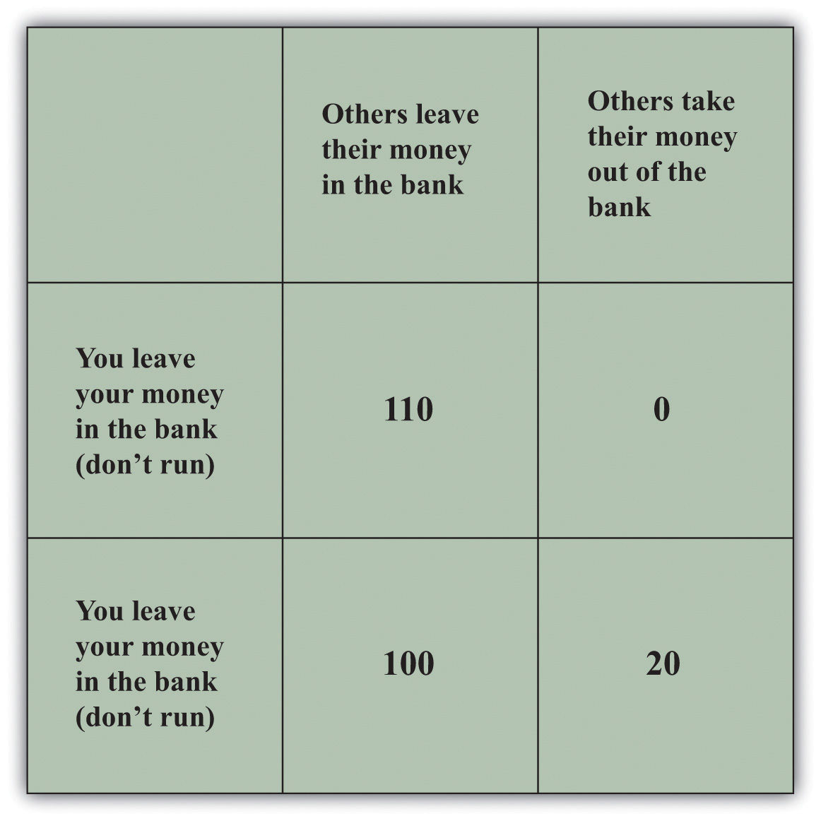
This table shows the payoffs in a bank-run game. That is, it shows you what you get back depending on your choice and everybody else’s choice about whether to run on the bank. If everyone else leaves money in the bank, then you should do the same, but if everyone else runs on the bank, you are better running as well.
Economists call this situation a coordination gameA strategic situation in which there are multiple equilibria.. In a coordination game, there are multiple equilibria. In this example, there is one equilibrium where there is no run on the bank, and there is another equilibrium where everyone runs to the bank to withdraw funds.
Toolkit: Section 31.18 "Nash Equilibrium"
You can find more details on coordination games in the toolkit.
During the Great Depression, a story such as this played out not only at one bank but at many. Figure 22.13 shows what happened in terms of the aggregate expenditure framework. Prior to the Great Depression, the economy was in a “high confidence” equilibrium, in which the banking system was healthy and confidence was high. Then—for some reason—people became nervous about leaving money in banks, and it became much harder for firms to obtain loans. The cost of borrowing—the real interest rateThe rate of return specified in terms of goods, not money.—increased, and investment decreased substantially. The planned spending line shifted downward, and the economy moved to the bad “low confidence” equilibrium. The downward shift in planned spending leads to a decrease in real GDP, given the existing level of prices.
Figure 22.13 should look familiar; it is the same as part (b) of Figure 22.10 "A Decrease in Aggregate Expenditures". This is because a decrease in autonomous consumption and a decrease in autonomous investment both look the same in the aggregate expenditure model, even though the underlying story is different. Of course, it is also possible that both autonomous consumption and autonomous investment decreased.
Figure 22.13
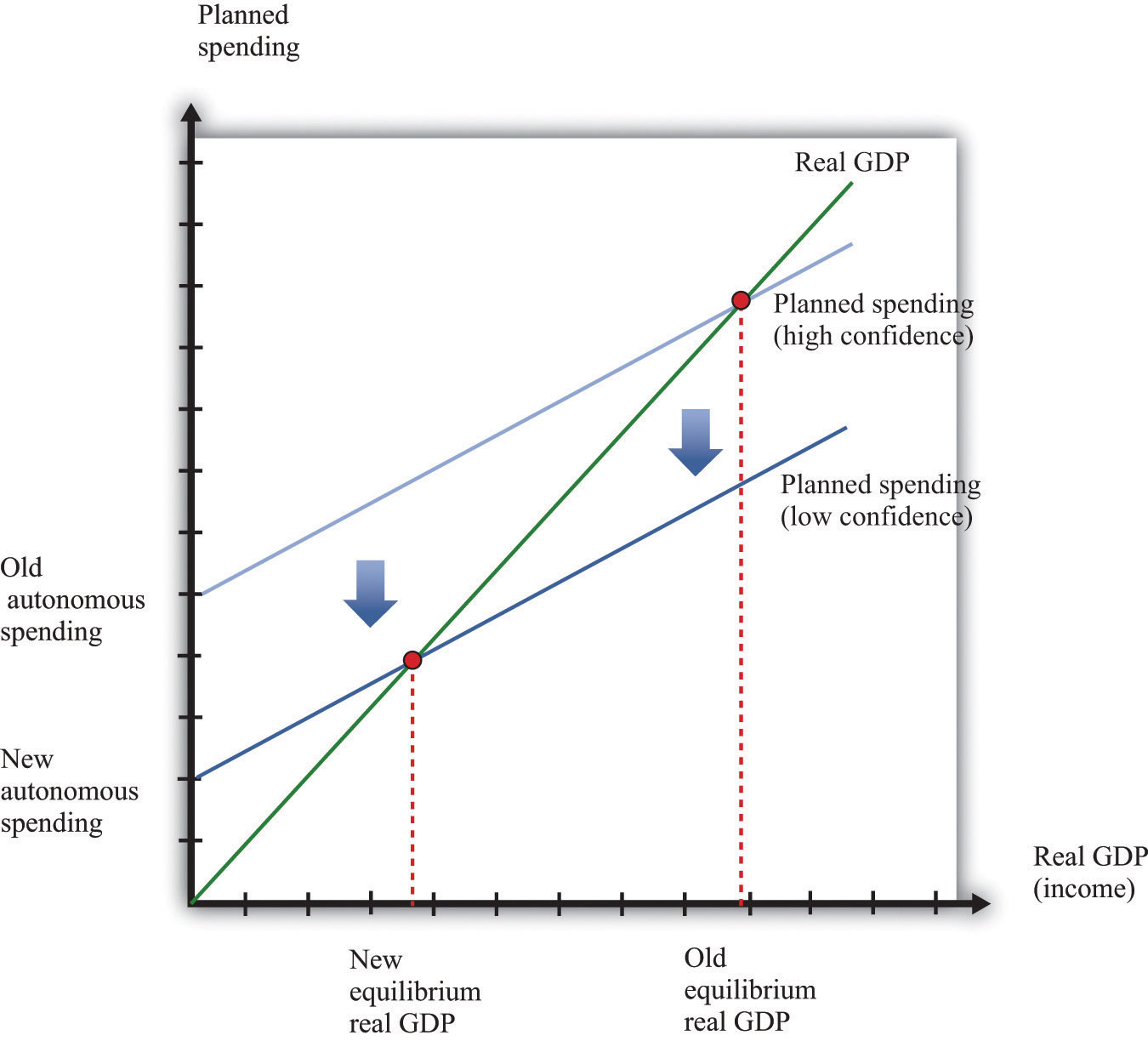
Failures in the financial sector lead to a drop in investment spending. During the Great Depression, a decrease in confidence in the banking system meant that many banks failed, and it became more difficult and expensive for firms to borrow. The planned spending line shifted downward, and real GDP decreased.
To summarize, the banking crisis made households reluctant to put money in the banks, and banks were reluctant to make loans. Two banking measures help us see what was happening. The currency-deposit ratioThe total amount of currency (banknotes plus coins) divided by the total amount of deposits in banks. is the total amount of currency (that is, either banknotes or coins) divided by the total amount of deposits in banks. The loan-deposit ratioThe total amount of loans made by banks divided by the total amount of deposits in banks. is the total amount of loans made by banks divided by the total amount of deposits in banks.
If the currency-deposit ratio is low, households are not holding very much cash but are instead keeping wealth in the form of bank deposits and other assets. The currency-deposit ratio increased from 0.09 in October 1929 to 0.23 in March 1933.See Milton Friedman and Anna Schwartz, A Monetary History of the United States, 1867–1960 (Princeton, NJ: Princeton University Press, 1963), Table B3. This means that households in the economy started holding onto cash rather than depositing it in banks. You can think of the loan-deposit ratio as a measure of the productivity of banks: banks take deposits and convert them into loans for investment. During the Great Depression, the loan-deposit ratio decreased from 0.86 to 0.73.See Ben Bernanke, “Nonmonetary Effects of the Financial Crisis in the Propagation of the Great Depression,” American Economic Review 73 (1983): 257–76, Table 1.
The story we have told explains why the economy departs from potential output but says nothing about how (if at all) the economy gets back to potential output. The answer is that prices have a tendency to adjust back toward their equilibrium levels, even if they do not always get there immediately. This is most easily understood by remembering that prices in the economy are, in the end, usually set by firms. When a firm sees a decrease in demand for its product, it does not necessarily decrease its prices immediately. Its decision about what price to choose depends on the prices of its inputs and the prices being set by its competitors. In addition, it depends on not only what those prices are right now but also what the firm expects to happen in the future. Deciding exactly what to do about prices can be a difficult decision for the managers of a firm.
Without analyzing this decision in detail, we can certainly observe that firms often keep prices fixed when demand decreases—at least to begin with. The result looks like that in Figure 22.6 "An Inward Shift in Market Demand for Houses". In the face of a prolonged decrease in demand, however, firms will lower prices. Some firms do this relatively quickly; others keep prices unchanged for longer periods. We conclude that prices are sticky; they do not decrease instantly, but they decrease eventually.Chapter 25 "Understanding the Fed" provides more detail about the price-adjustment decisions of firms. For the economy as a whole, this adjustment of prices is represented by a price-adjustment equationAn equation that describes how prices adjust in response to the output gap, given autonomous inflation..
Toolkit: Section 31.31 "Price Adjustment"
The difference between potential output and actual output is called the output gapThe difference between potential output and actual output.:
output gap = potential real GDP − actual real GDP.If an economy is in recession, the output gap is positive. If an economy is in a boom, then the output gap is negative. The inflation rate when an economy is at potential output (that is, when the output gap is zero) is called autonomous inflationThe level of inflation when the output gap is zero.. The overall inflation rate depends on both autonomous inflation and the output gap, as shown in the price-adjustment equation:
inflation rate = autonomous inflation − inflation sensitivity × output gap.This equation tells us that there are two reasons for increasing prices.
When real GDP is above potential output, there is upward pressure on prices in the economy. The inflation rate exceeds autonomous inflation. By contrast, when real GDP is below potential, there is downward pressure on prices. The inflation rate is below the autonomous inflation rate. The price-adjustment equation is shown in Figure 22.14 "Price Adjustment".
Figure 22.14 Price Adjustment
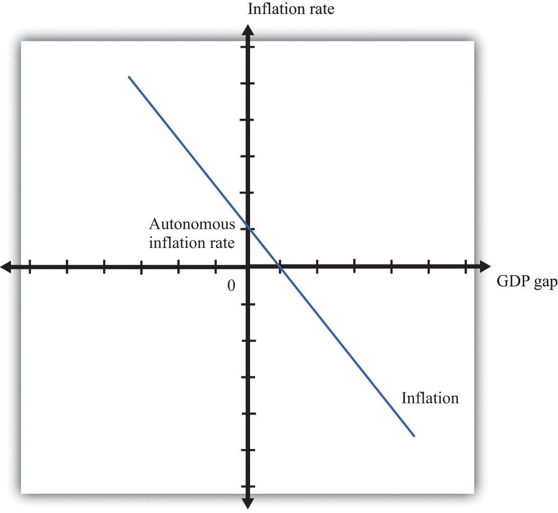
When an economy is in a recession, actual inflation is lower than autonomous inflation. In a boom, inflation is higher than its autonomous level.
We can apply this pricing equation to the Great Depression. Imagine first that autonomous inflation is zero. In this case, prices decrease when output is below potential. From 1929 to 1933, output was surely below potential and, as the equation suggests, this was a period of decreasing prices. After 1933, as the economy rebounded, the increase in the level of economic activity was matched with positive inflation—that is, increasing prices. This turnaround in inflation occurred even though the economy was still operating at a level below potential output. To match this movement in prices, we need to assume that—for some reason that we have not explained—autonomous inflation became positive in this period.
After you have read this section, you should be able to answer the following questions:
Understanding why the Great Depression occurred is certainly progress. But policymakers also wanted to know if there was anything that could be done in the face of this economic catastrophe. One of Keynes’ most lasting contributions to economics is that he showed how different kinds of economic policy could be used to assist economies that were stuck in recessions.
When markets are doing a good job of allocating resources, standard economic reasoning suggests that it is better for the government to stay out of the way. But when markets fail to allocate resources well, the government might be able to improve the overall functioning of the economy. The idea that markets left alone would coordinate aggregate economic activity is difficult to defend in the face of 25 percent unemployment of the labor force and a decline in economic activity of nearly 30 percent over a 4-year period. Thus the rationale for government intervention in the aggregate economy is that markets are failing to allocate resources properly, perhaps because prices and wages are sticky.
In the wake of the Great Depression, economists started advocating the use of government policy to improve the functioning of the macroeconomy. There are two kinds of government policy. Monetary policyChanges in interest rates and other tools that are under the control of the monetary authority of a country (the central bank). refers to changes in interest rates and other tools that are under the control of the monetary authority of a country (the central bank). Fiscal policyChanges in taxation and the level of government purchases, typically under the control of a country’s lawmakers. refers to changes in taxation and the level of government purchases; such policies are typically under the control of a country’s lawmakers. Stabilization policyThe use of monetary and fiscal policies to prevent large fluctuations in real GDP. is the general term for the use of monetary and fiscal policies to prevent large fluctuations in real gross domestic product (real GDP).
In the United States, the Federal Reserve Bank controls monetary policy, and fiscal policy is controlled by the president, the Congress, and state governments. In the countries of the European Union, monetary policy is controlled by the European Central Bank, and fiscal policies are controlled by the individual governments of the member countries.
Keynes suggested that the cause of the Great Depression was an unusually low level of aggregate spending. This diagnosis suggests an immediate remedy: use government policies to increase aggregate spending. Because
change in GDP = multiplier × change in autonomous spending,any government policy that increases autonomous spending will, through this equation, also increase GDP. There are many different policies at the disposal of the government, but they are similar at heart. The idea is to stimulate one of the components of aggregate spending—consumption, investment, government purchases, or net exports.
One fiscal policy measure is an increase in government purchases. Suppose the government increases its expenditure—perhaps by hiring more teachers, buying more tanks, or building more roads. This increases autonomous spending and works its way through the economy, just as in our earlier discussion of a decrease in autonomous consumption—except now we are talking about an increase rather than a decrease. If the government spends an extra dollar, this immediately expands income by that dollar. Extra income leads to extra spending, which leads to further increases in output and income. The process continues around and around the circular flow.
Imagine that, as before, the marginal propensity to spend is 0.8, so that the multiplier is 5. If the government increases expenditure on goods and services by $1 billion, overall GDP in the economy will increase by $5 billion. Thus to offset the decrease in real GDP of about $90 billion between 1929 and 1933, assuming a marginal propensity to spend of 0.8, the federal government should have increased government spending by $18 billion. The multiplier is a double-edged sword. It has the bad effect that it can turn small decreases in spending into big decreases in output. But it also means that relatively small changes in government spending can have a big effect on output.
Tax cuts are another way to stimulate the economy. If households have to pay fewer taxes to the government, they are likely to spend more on consumption goods. This form of policy intervention has been used over and over again by governments in the United States and elsewhere. Tax cuts, like government spending, must be paid for. If the government spends more and taxes less, then the government deficit increases. The government must borrow to finance such fiscal policy measures.Chapter 27 "Income Taxes" and Chapter 29 "Balancing the Budget" have more to say about fiscal policy.
The central bank can use monetary policy to affect aggregate spending. Monetary policy operates through changes in interest rates, which are—in the short run at least—under the influence of the central bank. Lower interest rates make it cheaper for firms to borrow, which encourages them to increase investment spending. Lower interest rates likewise mean lower mortgage rates, so households are more likely to buy new homes. Lower interest rates may encourage households to borrow and spend more on other goods. And lower interest rates can even encourage net exports.The link from interest rates to net exports is complicated because it involves changes in exchange rates. You do not need to worry here about how it works. We explain it, together with other details of monetary policy, in Chapter 25 "Understanding the Fed".
We have argued that monetary and fiscal policies could have been used to help the economy out of the Great Depression. But what did policymakers actually do at the time? The answer comes in two parts: at the start of the Great Depression, they did not do much; after 1932, they did rather more.
Both presidential candidates campaigned in favor of conservative fiscal policy in 1932. Here are some excerpts from the party platforms.See John Woolley and Gerhard Peters, The American Presidency Project, accessed June 30, 2011, http://www.presidency.ucsb.edu.
From the Democratic Party platform:
We advocate an immediate and drastic reduction of governmental expenditures by abolishing useless commissions and offices, consolidating departments and bureaus, and eliminating extravagance to accomplish a saving of not less than twenty-five per cent in the cost of the Federal Government. And we call upon the Democratic Party in the states to make a zealous effort to achieve a proportionate result.
We favor maintenance of the national credit by a federal budget annually balanced on the basis of accurate executive estimates within revenues, raised by a system of taxation levied on the principle of ability to pay.“Democratic Party Platform of 1932,” The American Presidency Project, accessed June 30, 2011, http://www.presidency.ucsb.edu/ws/index.php?pid=29595#ax zz1N9yDnpSR.
From the Republican Party platform:
The President’s program contemplates an attack on a broad front, with far-reaching objectives, but entailing no danger to the budget. […]
Constructive plans for financial stabilization cannot be completely organized until our national, State and municipal governments not only balance their budgets but curtail their current expenses as well to a level which can be steadily and economically maintained for some years to come.“Republican Party Platform of 1932,” The American Presidency Project, accessed June 30, 2011, http://www.presidency.ucsb.edu/ws/index.php?pid=29638#axz z1N9yDnpSR.
Both parties were arguing for cuts in government expenditures, not the increases that (with the benefit of hindsight and better theory) we have suggested were needed. Monetary policy was likewise not used to stimulate the economy at this time. It seems unlikely that the fiscal and monetary authorities knew what to do but did nothing. Instead, the tools of economic thought needed to guide policy were simply not sufficiently well developed at the time. In keeping with the prevailing view that the economy was self-correcting, the incumbent Republican president, Herbert Hoover, had insisted that “prosperity is just around the corner.”
The election of Franklin Roosevelt in 1932 was a turning point. After his election, President Roosevelt and his advisors created a series of measures—called the New Deal—that were intended to stabilize the economy. In terms of fiscal policy, the US government moved away from budget balance and adopted a much more aggressive spending policy. Government spending increased from 3.2 percent of real GDP in 1932 to 9.3 percent of GDP by 1936. These spending increases were financed by budget deficits.
Roosevelt also took action to stabilize the banking system, most notably by creating a system of deposit insurance. This policy remains with us today: if you have deposits in a US bank, the federal government insures them. According to the Federal Deposit Insurance Corporation (http://www.fdic.gov), not a single depositor has lost a cent since the introduction of deposit insurance.The FDIC site (http://www.fdic.gov) provides a discussion the history of this fund and current activities. The discussion of “Who is the FDIC?” (http://www.fdic.gov/about/learn/symbol/index.html) is a good place to start. Finally, the 1930s was also the time of the introduction of Social Security and other measures to protect workers. The Social Security Administration (http://www.ssa.gov) originated in 1935.General information on social security is available at http://www.ssa.gov. The history of the legislation, including various House and Senate Bills, is also available at http://www.ssa.gov/history/history.html. The original act included old-age benefits and the provision of unemployment insurance. The disability part of the program was created in 1956.
The New Deal brought about changes not only in policy but also in attitudes toward policymaking. Gardiner Means, who was an economic adviser to the Roosevelt administration in 1933, said of policymaking at the time:
It was this which produced the yeastiness of experimentation that made the New Deal what it was. A hundred years from now, when historians look back on this, they will say a big corner was turned. People agreed old things didn’t work. What ran through the whole New Deal was finding a way to make things work.
Before that, Hoover would loan money to farmers to keep their mules alive, but wouldn’t loan money to keep their children alive. This was perfectly right within the framework of classical thinking. If an individual couldn’t get enough to eat, it was because he wasn’t on the ball. It was his responsibility. The New Deal said: “Anybody who is unemployed isn’t necessarily unemployed because he is shiftless.”See Studs Terkel, Hard Times: An Oral History of the Great Depression (New York: Pantheon Books, 1970), 247.
We started this chapter by describing the experience of the economy of the United States and other countries in the 1930s. The catastrophic economic performance of that period was difficult to reconcile with the view of classical economists that markets always worked to coordinate aggregate economic activity. Although technological progress provides a plausible explanation of the roaring twenties, technological regress is much less convincing as a story of the Great Depression. Technological regress also cannot explain the behavior of the price level and real wages during the Great Depression.
The Keynesian view explains the Great Depression as being driven by a decrease in aggregate spending, caused primarily by two factors: household consumption decreased because the stock market crash reduced household wealth, and investment decreased because of disruption of the financial intermediation process and pessimism over the future of the economy. These reductions in spending, through the multiplier, led to large reductions in real output. This story is consistent with the observed reductions in consumption, investment, and real GDP. With sticky prices, these reductions in spending translate into lower real GDP. The simple Keynesian story also has two problems: it can explain increasing prices only by assuming an exogenous increase in autonomous inflation and it provides no explanation of why observed technology decreased in the Great Depression period.
Along with the Keynesian explanation of the Great Depression comes a solution: use government policies to manage aggregate spending. If the aggregate expenditure model were literally true, policymaking would become an exact science: the policymaker would start with a target level of output and then determine the level of, say, government purchases needed to reach that target. As you might imagine, life as an economic policymaker is more complicated. The economists and politicians designing fiscal and monetary policy do not have a perfect picture of the current state of the economy. Moreover, control over policy tools is often inexact, and policy decisions take time.
The Great Depression remains something of a puzzle to macroeconomists. This became very apparent again recently during the so-called Great Recession—the major economic downturn that began in 2008. There are some resemblances between the two episodes, and the experience of the Great Depression certainly influenced some of the monetary policy decisions that were made in recent years. In this chapter, we did not yet consider monetary policy in detail. Chapter 25 "Understanding the Fed", which discusses the conduct of monetary policy, also addresses monetary policy during the Great Depression.
The aggregate expenditure framework is not a very sophisticated theory of the economy. Much work in macroeconomics in the decades since the Great Depression has involved refining the various pieces of the aggregate expenditure model. Economists have developed more rigorous theories of consumption, investment, and price adjustment, for example, in which they emphasize how households and firms base their decisions on expectations about the future. But Keynes’ fundamental insight—that the level of output may sometimes be determined not by the productive capacity of the economy but by the overall level of spending—remains at the heart of macroeconomic research and policymaking today.
Photo exhibits about the Great Depression:
Spreadsheet Exercises
Economics Detective


