In the goods market model, it is assumed that the exchange rate (E$/£) is directly related to current account demand in the United States. The logic of the relationship goes as follows. If the dollar depreciates, meaning E$/£ rises, then foreign goods will become more expensive to U.S. residents, causing a decrease in import demand. At the same time U.S. goods will appear relatively cheaper to foreign residents, causing an increase in demand for U.S. exports. The increase in export demand and decrease in import demand both contribute to an increase in the current account demand. Since in the goods market model, any increase in demand results in an increase in supply to satisfy that demand, the dollar depreciation should also lead to an increase in the actual current account balance.
In real-world economies, however, analysis of the data suggests that in many instances a depreciating currency tends to cause, at least, a temporary increase in the deficit rather than the predicted decrease. The explanation for this temporary reversal of the cause-and-effect relationship is called the J-curve theory. In terms of future use of the AA-DD model, we will always assume the J-curve effectA theory that suggests that after a currency depreciation, the current account balance will first fall for a period of time before beginning to rise as is normally expected. is not operating, unless otherwise specified. One should think of this effect as a possible short-term exception to the standard theory.
The theory of the J-curve is an explanation for the J-like temporal pattern of change in a country’s trade balance in response to a sudden or substantial depreciation (or devaluation) of the currency.
Consider Figure 8.6 "J-Curve Effect", depicting two variables measured, hypothetically, over some period: the U.S. dollar / British pound (E$/£) and the U.S. current account balance (CA = EX − IM). The exchange rate is meant to represent the average value of the dollar against all other trading country currencies and would correspond to a dollar value index that is often constructed and reported. Since the units of these two data series would be in very different scales, we imagine the exchange rate is measured along the left axis, while the CA balance is measured in different units on the right-hand axis. With appropriately chosen scales, we can line up the two series next to each other to see whether changes in the exchange rate seem to correlate with positive or negative changes in the CA balance.
Figure 8.6 J-Curve Effect
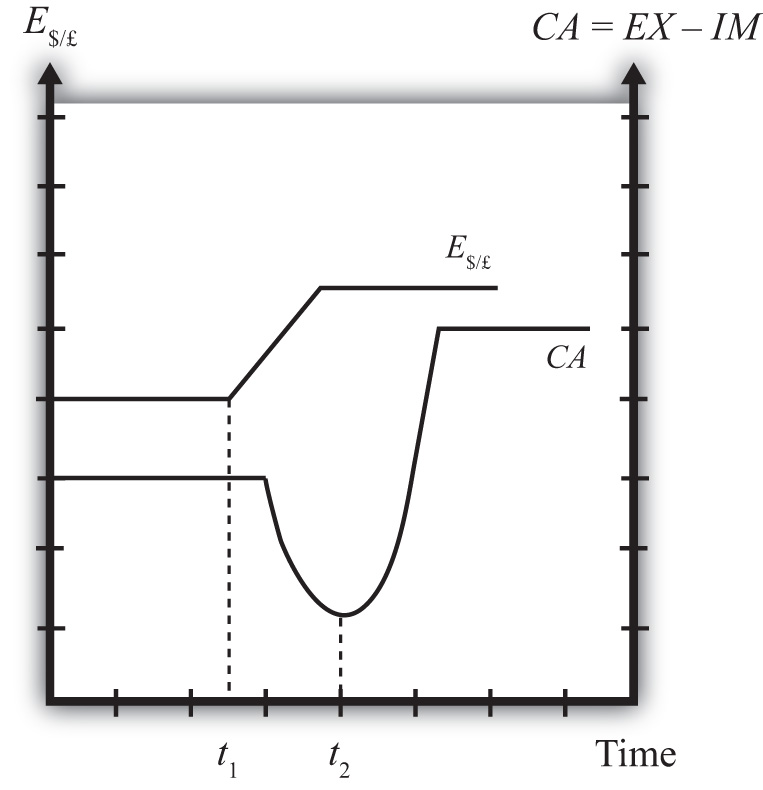
As previously mentioned, the standard theory suggests a positive relationship between E$/£ and the U.S. current account, implying that, ceteris paribus, any dollar depreciation (an increase in E$/£) should cause an increase in the CA balance.
However, what sometimes happens instead, is immediately following the dollar depreciation at time t1, the CA balance falls for a period of time, until time t2 is reached. In this phase, a CA deficit would become larger, not smaller.
Eventually, after period t2, the CA balance reverses direction and begins to increase—in other words, a trade deficit falls. The diagram demonstrates clearly how the CA balance follows the pattern of a “J” in the transition following a dollar depreciation, hence the name J-curve theory.
In the real world, the period of time thought necessary for the CA balance to traverse the J pattern is between one and two years. However, this estimate is merely a rough rule of thumb as the actual paths will be influenced by many other variable changes also occurring at the same time. Indeed, in some cases the J-curve effect may not even arise, so there is nothing automatic about it.
The reasons for the J-curve effect can be better understood by decomposing the current account balance. The basic definition of the current account is the difference between the value of exports and the value of imports. That is,
CA = EX − IM.The current account also includes income payments and receipts and unilateral transfers, but these categories are usually small and will not play a big role in this discussion—so we’ll ignore them. The main thing to take note about this definition is that the CA is measured in “value” terms, which means in terms of dollars. The way these values are determined is by multiplying the quantity of imports by the price of each imported item. We expand the CA definition by using the summation symbol and imagining summing up across all exported goods and all imported goods:
CA = ΣPEXQEX − ΣPIMQIM.Here ΣPEXQEX represents the summation of the price times quantities of all goods exported from the country, while ΣPEXQEX is the summation of the price times quantities of all goods imported from the country.
However, for imported goods we could also take note that foreign products are denominated in foreign currency terms. To convert them to U.S. dollars we need to multiply by the current spot exchange rate. Thus we can expand the CA definition further by incorporating the exchange rate into the import term as follows:
CA = ΣPEXQEX − ΣE$/£P*IMQIM.Here E$/£ represents whatever dollar/pound rate prevailed at the time of imports, and PIM* represents the price of each imported good denominated in foreign (*) pound currency terms. Thus the value of imports is really the summation across all foreign imports of the exchange rate times the foreign price times quantity.
The J-curve theory recognizes that import and export quantities and prices are often arranged in advance and set into a contract. For example, an importer of watches is likely to enter into a contract with the foreign watch company to import a specific quantity over some future period. The price of the watches will also be fixed by the terms of the contract. Such a contract provides assurances to the exporter that the watches he makes will be sold. It provides assurances to the importer that the price of the watches will remain fixed. Contract lengths will vary from industry to industry and firm to firm, but may extend for as long as a year or more.
The implication of contracts is that in the short run, perhaps over six to eighteen months, both the local prices and quantities of imports and exports will remain fixed for many items. However, the contracts may stagger in time—that is, they may not all be negotiated and signed at the same date in the past. This means that during any period some fraction of the contracts will expire and be renegotiated. Renegotiated contracts can adjust prices and quantities in response to changes in market conditions, such as a change in the exchange rate. Thus in the months following a dollar depreciation, contract renegotiations will gradually occur, causing eventual, but slow, changes in the prices and quantities traded.
With these ideas in mind, consider a depreciation of the dollar. In the very short run—say, during the first few weeks—most of the contract terms will remain unchanged, meaning that the prices and quantities of exports and imports will also stayed fixed. The only change affecting the CA formula, then, is the increase in E$/*. Assuming all importers have not hedged their trades by entering to forward contracts, the increase in E$/* will result in an immediate increase in the value of imports measured in dollar terms. Since the prices and quantities do not change immediately, the CA balance falls. This is what can account for the initial stage of the J-curve effect, between periods t1 and t2.
As the dollar depreciation continues, and as contracts begin to be renegotiated, traders will adjust quantities demanded. Since the dollar depreciation causes imported goods to become more expensive to U.S. residents, the quantity of imported goods demanded and purchased will fall. Similarly, exported goods will appear cheaper to foreigners, and so as their contracts are renegotiated, they will begin to increase demand for U.S. exports. The changes in these quantities will both cause an increase in the current account (decrease in a trade deficit). Thus, as several months and years pass, the effects from the changes in quantities will surpass the price effect caused by the dollar depreciation and the CA balance will rise as shown in the diagram after time t2.
It is worth noting that the standard theory, which says that a dollar depreciation causes an increase in the current account balance, assumes that the quantity effects—that is, the effects of the depreciation on export and import demand—are the dominant effects. The J-curve theory qualifies that effect by suggesting that although the quantity or demand effects will dominate, it may take several months or years before becoming apparent.
Jeopardy Questions. As in the popular television game show, you are given an answer to a question and you must respond with the question. For example, if the answer is “a tax on imports,” then the correct question is “What is a tariff?”


