Eating a french fry makes most people a little bit happier, and most people are willing to give up something of value—a small amount of money or a little bit of time—to eat one. The personal value of the french fry is measured by what one is willing to give up to eat it. That value, expressed in dollars, is the willingness to pay for french fries. So, if you are willing to give up 3 cents for a single french fry, your willingness to pay is 3 cents. If you pay a penny for the french fry, you’ve obtained a net of 2 cents in value. Those 2 cents—the difference between your willingness to pay and the amount you pay—is known as consumer surplusThe value of consuming a good, minus the price paid.. Consumer surplus is the value of consuming a good, minus the price paid.
The value of items—like french fries, eyeglasses, or violins—is not necessarily close to what one must pay for them. For people with bad vision, eyeglasses might be worth $10,000 or more in the sense that people would be willing to pay this amount or more to wear them. Since one doesn’t have to pay nearly this much for eyeglasses means that the consumer surplus derived from eyeglasses is enormous. Similarly, an order of french fries might be worth $3 to a consumer, but since they are available for $1, the consumer obtains a surplus of $2 from purchase.
How much is a second order of french fries worth? For most of us, the first order is worth more than the second one. If a second order is worth $2, we would still gain from buying it. Eating a third order of fries is worth less still, and at some point we’re unable or unwilling to eat any more fries even when they are free, that implies that the value of additional french fries becomes zero eventually.
We will measure consumption generally as units per period of time, for example, french fries consumed per month.
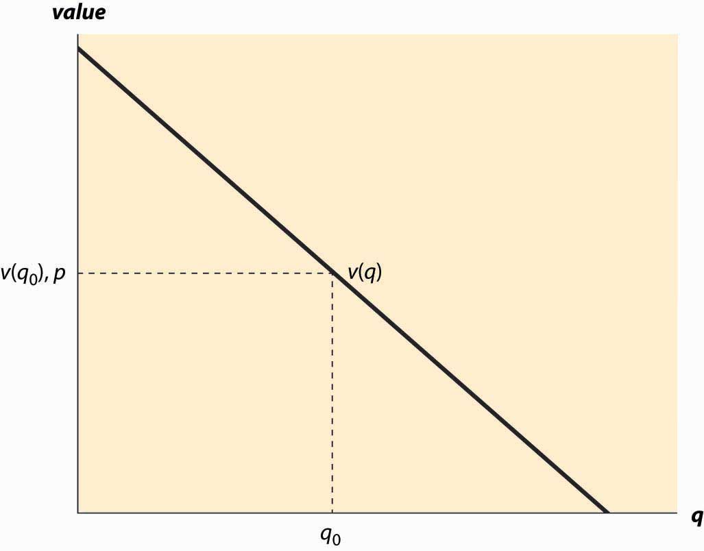
Many, but not all, goods have this feature of diminishing marginal valueCondition in which the value of the last unit declines as the number consumed rises.—the value of the last unit declines as the number consumed rises. If we consume a quantity q, that implies the marginal value, denoted by v(q), falls as the number of units rise.When marginal value falls, which may occur with beer consumption, constructing demand takes some additional effort, which isn’t a great deal of consequence. Buyers will still choose to buy a quantity where marginal value is decreasing. An example is illustrated in Figure 2.1 "The demand curve", where the value is a straight line, declining in the number of units.
Figure 2.1 The demand curve

Demand needn’t be a straight line, and indeed could be any downward-sloping curve. Contrary to the usual convention, the quantity demanded for any price is represented by the vertical axis whereas the price is plotted along the horizontal.
It is often important to distinguish the demand curve—the relationship between price and quantity demanded—from the quantity demanded. Typically, “demand” refers to the curve, while “quantity demanded” is a point on the curve.
For a price p, a consumer will buy units q such that v(q) > p since those units are worth more than they cost. Similarly, a consumer would not buy units for which v(q) < p. Thus, the quantity q0 that solves the equation v(q0) = p indicates the quantity the consumer will buy. This value is illustrated in Figure 2.1 "The demand curve".We will treat units as continuous, even though they are discrete units. This simplifies the mathematics; with discrete units, the consumer buys those units with value exceeding the price and doesn’t buy those with value less than the price, just as before. However, since the value function isn’t continuous, much less differentiable, it would be an accident for marginal value to equal price. It isn’t particularly difficult to accommodate discrete products, but it doesn’t enhance the model so we opt for the more convenient representation. Another way of expressing this insight is that the marginal value curve is the inverse of the demand function, where the demand function gives the quantity purchased at a given price. Formally, if x(p) is the quantity a consumer buys at price p, then
But what is the marginal value curve? Suppose the total value of consumption is u(q). A consumer who pays u(q) for the quantity q is indifferent to receiving nothing and paying nothing. For each quantity, there should exist one and only one price that makes the consumer indifferent between purchasing and receiving nothing. If the consumer is just willing to pay u(q), any additional amount exceeds what the consumer should be willing to pay.
The consumer facing price p receives consumer surplus of CS = u(q) – pq. In order to obtain the maximal benefit, the consumer chooses q to maximize u(q) – pq. When the function CS is maximized, its derivative is zero. This implies that the quantity maximizing the consumer surplus must satisfy
Thus, implying that the marginal value is the derivative of the total value.
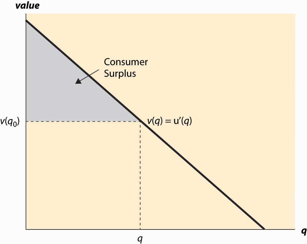
Consumer surplus is the value of the consumption minus the amount paid, and it represents the net value of the purchase to the consumer. Formally, it is u(q) – pq. A graph of consumer surplus is generated by the following identity:
This expression shows that consumer surplus can be represented as the area below the demand curve and above the price, as illustrated in Figure 2.2 "Consumer surplus". The consumer surplus represents the consumer’s gains from trade, the value of consumption to the consumer net of the price paid.
Figure 2.2 Consumer surplus

The consumer surplus can also be expressed using the demand curve, by integrating from the price up to where the demand curve intersects with the price axis. In this case, if x(p) is demand, we have
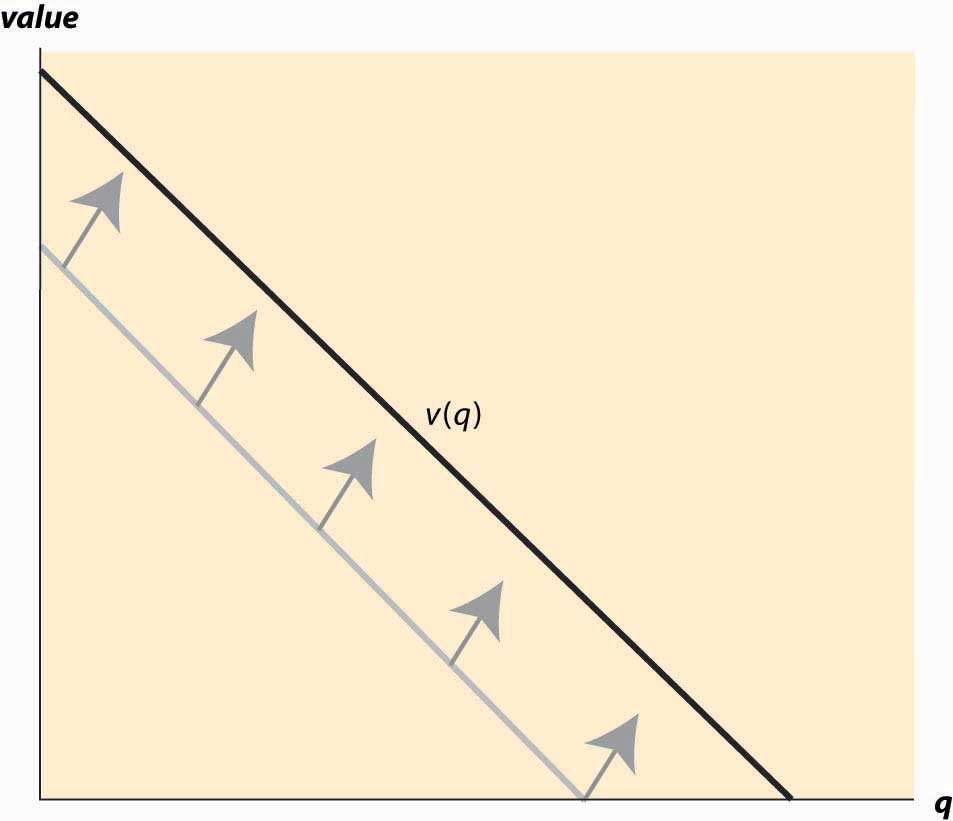
When you buy your first car, you experience an increase in demand for gasoline because gasoline is pretty useful for cars and not so much for other things. An imminent hurricane increases the demand for plywood (to protect windows), batteries, candles, and bottled water. An increase in demand is represented by a movement of the entire curve to the northeast (up and to the right), which represents an increase in the marginal value v (movement up) for any given unit, or an increase in the number of units demanded for any given price (movement to the right). Figure 2.3 "An increase in demand" illustrates a shift in demand.
Similarly, the reverse movement represents a decrease in demand. The beauty of the connection between demand and marginal value is that an increase in demand could, in principle, have meant either more units demanded at a given price or a higher willingness to pay for each unit, but those are in fact the same concept. Both changes create a movement up and to the right.
For many goods, an increase in income increases the demand for the good. Porsche automobiles, yachts, and Beverly Hills homes are mostly purchased by people with high incomes. Few billionaires ride the bus. Economists aptly named goods whose demand doesn’t increase with income inferior goodsGoods whose demand don’t increase with income., with the idea that people substitute to better quality, more expensive goods as their incomes rise. When demand for a good increases with income, the good is called a normal goodGoods whose demand increases with income.. It would have been better to call such goods superior, but it is too late to change such a widely accepted convention.
Figure 2.3 An increase in demand

Another factor that influences demand is the price of related goods. The dramatic fall in the price of computers over the past 20 years has significantly increased the demand for printers, monitors, and Internet access. Such goods are examples of complementsFor a given good x, a good whose consumption increases the value of x.. Formally, for a given good x, a complement is a good whose consumption increases the value of x. Thus, the use of computers increases the value of peripheral devices like printers and monitors. The consumption of coffee increases the demand for cream for many people. Spaghetti and tomato sauce, national parks and hiking boots, air travel and hotel rooms, tables and chairs, movies and popcorn, bathing suits and sunscreen, candy and dentistry—all are examples of complements for most people. Consumption of one increases the value of the other. The complementary relationship is typically symmetric—if consumption of x increases the value of y, then consumption of y must increase the value of x.The basis for this insight can be seen by denoting the total value in dollars of consuming goods x and y as u(x, y). Then the demand for x is given by the partial The statement that y is a complement means that the demand for x rises as y increases; that is, But then with a continuous second derivative, , which means the demand for y, increases with x. From this we can predict that if the price of good y decreases, then the amount good y, a complementary good to x, will decline. Why, you may ask? The reason is that consumers will purchase more of good x when its price decreases. This will make good y more valuable, and hence consumers will also purchase more of good y as a result.
The opposite case of a complement is a substituteFor a given good x, a good whose consumption decreases the value of x.. For a given good x, a substitute is a good whose consumption decreases the value of x. Colas and root beer are substitutes, and a fall in the price of root beer (resulting in an increase in the consumption of root beer) will tend to decrease the demand for colas. Pasta and ramen, computers and typewriters, movies (in theaters) and sporting events, restaurants and dining at home, spring break in Florida versus spring break in Mexico, marijuana and beer, economics courses and psychology courses, driving and bicycling—these are all examples of substitutes for most people. An increase in the price of a substitute increases the demand for a good; and, conversely, a decrease in the price of a substitute decreases demand for a good. Thus, increased enforcement of the drug laws, which tends to increase the price of marijuana, leads to an increase in the demand for beer.
Much of demand is merely idiosyncratic to the individual—some people like plaids, some like solid colors. People like what they like. People often are influenced by others—tattoos are increasingly common, not because the price has fallen but because of an increased acceptance of body art. Popular clothing styles change, not because of income and prices but for other reasons. While there has been a modest attempt to link clothing style popularity to economic factors,Skirts are allegedly shorter during economic booms and lengthen during recessions. by and large there is no coherent theory determining fads and fashions beyond the observation that change is inevitable. As a result, this course, and economics generally, will accept preferences for what they are without questioning why people like what they like. While it may be interesting to understand the increasing social acceptance of tattoos, it is beyond the scope of this text and indeed beyond most, but not all, economic analyses. We will, however, account for some of the effects of the increasing acceptance of tattoos through changes in the number of parlors offering tattooing, changes in the variety of products offered, and so on.
Suppose the demand for wheat is given by qd = 3 – p and the supply of wheat is given by qs = 2p, where p is the price.
How will the following affect the price of a regular cup of coffee, and why?
| Slices of pizza | Total value |
|---|---|
| 0 | 0 |
| 1 | 4 |
| 2 | 7 |
| 3 | 10 |
| 4 | 12 |
| 5 | 11 |