Consider an entrepreneur who would like to maximize profit, perhaps by running a delivery service. The entrepreneur uses two inputs, capital K (e.g., trucks) and labor L (e.g., drivers), and rents the capital at cost r per dollar of capital. The wage rate for drivers is w. The production function is F(K, L)—that is, given inputs K and L, the output is F(K, L). Suppose p is the price of the output. This gives a profit ofEconomists often use the symbol π, the Greek letter “pi,” to stand for profit. There is little risk of confusion because economics doesn’t use the ratio of the circumference to the diameter of a circle very often. On the other hand, the other two named constants, Euler’s e and i, the square root of -1, appear fairly frequently in economic analysis.
First, consider the case of a fixed level of K. The entrepreneur chooses L to maximize profit. The value L* of L that maximizes the function π must satisfy
This expression is known as a first-order conditionA mathematical condition for optimization stating that the first derivative is zero., a mathematical condition for optimization stating that the first derivative is zero.It is possible that L = 0 is the best that an entrepreneur can do. In this case, the derivative of profit with respect to L is not necessarily zero. The first-order condition instead would be either or L = 0, and The latter pair of conditions reflects the logic that either the derivative is zero and we are at a maximum, or L = 0, in which case a small increase in L must not cause π to increase. The first-order condition recommends that we add workers to the production process up to the point where the last worker’s marginal product is equal to his wage (or cost).
Figure 9.4 Profit-maximizing labor input
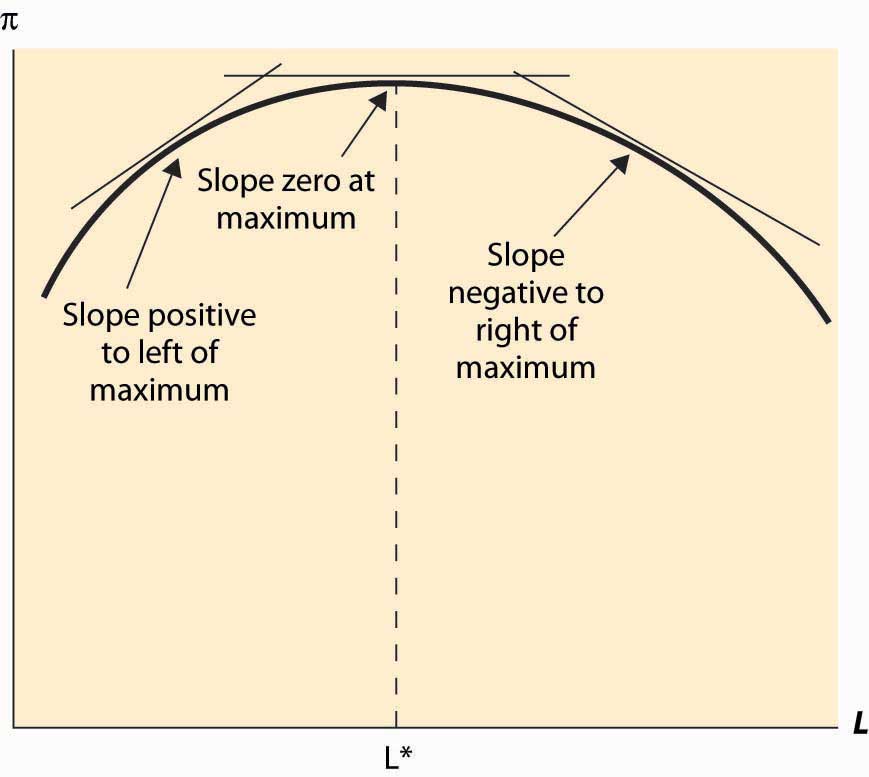
In addition, a second characteristic of a maximum is that the second derivative is negative (or nonpositive). This arises because, at a maximum, the slope goes from positive (since the function is increasing up to the maximum) to zero (at the maximum) to being negative (because the function is falling as the variable rises past the maximum). This means that the derivative is falling or that the second derivative is negative. This logic is illustrated in Figure 9.4 "Profit-maximizing labor input".
The second property is known as the second-order conditionA mathematical condition for maximization stating that the second derivative is nonpositive., a mathematical condition for maximization stating that the second derivative is nonpositive.The orders refer to considering small, but positive, terms Δ, which are sent to zero to reach derivatives. The value Δ2, the second-order term, goes to zero faster than Δ, the first-order term. It is expressed as
This is enough of a mathematical treatment to establish comparative statics on the demand for labor. Here we treat the choice L* as a function of another parameter—the price p, the wage w, or the level of capital K. For example, to find the effect of the wage on the labor demanded by the entrepreneur, we can write
This expression recognizes that the choice L* that the entrepreneur makes satisfies the first-order condition and results in a value that depends on w. But how does it depend on w? We can differentiate this expression to obtain
or
The second-order condition enables one to sign the derivative. This form of argument assumes that the choice L* is differentiable, which is not necessarily true.
Digression: In fact, there is a form of argument that makes the point without calculus and makes it substantially more general. Suppose w1 < w2 are two wage levels and that the entrepreneur chooses L1 when the wage is w1 and L2 when the wage is w2. Then profit maximization requires that these choices are optimal. In particular, when the wage is w1, the entrepreneur earns higher profit with L1 than with L2:
When the wage is w2, the entrepreneur earns higher profit with L2 than with L1:
The sum of the left-hand sides of these two expressions is at least as large as the sum of the right-hand side of the two expressions:
A large number of terms cancel to yield the following:
This expression can be rearranged to yield the following:
This shows that the higher labor choice must be associated with the lower wage. This kind of argument, sometimes known as a revealed preferenceKind that states that choice implies preference. kind of argument, states that choice implies preference. It is called “revealed preference” because choices by consumers were the first place the type of argument was applied. It can be very powerful and general, because issues of differentiability are avoided. However, we will use the more standard differentiability-type argument, because such arguments are usually more readily constructed.
The effect of an increase in the capital level K on the choice by the entrepreneur can be calculated by considering L* as a function of the capital level K:
Differentiating this expression with respect to K, we obtain
or
We know the denominator of this expression is not positive, thanks to the second-order condition, so the unknown part is the numerator. We then obtain the conclusion that
an increase in capital increases the labor demanded by the entrepreneur if and decreases the labor demanded if
This conclusion looks like gobbledygook but is actually quite intuitive. Note that means that an increase in capital increases the derivative of output with respect to labor; that is, an increase in capital increases the marginal product of labor. But this is, in fact, the definition of a complement! That is, means that labor and capital are complements in production—an increase in capital increases the marginal productivity of labor. Thus, an increase in capital will increase the demand for labor when labor and capital are complements, and it will decrease the demand for labor when labor and capital are substitutes.
This is an important conclusion because different kinds of capital may be complements or substitutes for labor. Are computers complements or substitutes for labor? Some economists consider that computers are complements to highly skilled workers, increasing the marginal value of the most skilled, but substitutes for lower-skilled workers. In academia, the ratio of secretaries to professors has fallen dramatically since the 1970s as more and more professors are using machines to perform secretarial functions. Computers have increased the marginal product of professors and reduced the marginal product of secretaries, so the number of professors rose and the number of secretaries fell.
The revealed preference version of the effect of an increase in capital is to posit two capital levels, K1 and K2, with associated profit-maximizing choices L1 and L2. The choices require, for profit maximization, that
and
Again, adding the left-hand sides together produces a result at least as large as the sum of the right-hand sides:
Eliminating redundant terms yields
or
or
Here we use the standard convention that
or
and finally
Thus, if K2 > K1 and for all K and L, then L2 ≥ L1; that is, with complementary inputs, an increase in one input increases the optimal choice of the second input. In contrast, with substitutes, an increase in one input decreases the other input. While we still used differentiability of the production function to carry out the revealed preference argument, we did not need to establish that the choice L* was differentiable to perform the analysis.
Example (Labor demand with the Cobb-Douglas production function): The Cobb-Douglas production function has the form for constants A, α, and β, all positive. It is necessary for β < 1 for the solution to be finite and well defined. The demand for labor satisfies
or
When α + β = 1, L is linear in capital. Cobb-Douglas production is necessarily complementary; that is, an increase in capital increases labor demanded by the entrepreneur.
The demand for hamburgers has a constant elasticity of 1 of the form x(p) = 8,000 p – 1. Each entrant in this competitive industry has a fixed cost of $2,000 and produces hamburgers per year, where x is the amount of meat in pounds.
A company that produces software needs two inputs, programmers (x) at a price of p and computers (y) at a price of r. The output is given by T = 4x1/3y1/3, measured in pages of code.
A toy factory costs $2 million to construct, and the marginal cost of the qth toy is max[10, q2/1,000].


