Over a long period of time, an entrepreneur can adjust both the capital and the labor used at the plant. This lets the entrepreneur maximize profit with respect to both variables K and L. We’ll use a double star, **, to denote variables in their long-run solution. The approach to maximizing profit over two c separately with respect to each variable, thereby obtaining the conditions
and
We see that, for both capital and labor, the value of the marginal product is equal to the purchase price of the input.
It is more challenging to carry out comparative statics exercises with two variables, and the general method won’t be developed here.If you want to know more, the approach is to arrange the two equations as a vector with x = (K, L), z = (r/p, w/p), so that and then differentiate to obtain which can then be solved for each comparative static. However, we can illustrate one example as follows.
Example: The Cobb-Douglas production function implies choices of capital and labor satisfying the following two first-order conditions:It is necessary for α + β < 1 for the solution to be finite and well defined.
To solve these expressions, first rewrite them to obtain
and
Then divide the first expression by the second expression to yield
or
This can be substituted into either equation to obtain
and
While these expressions appear complicated, the dependence on the output price p, and the input prices r and w, is quite straightforward.
How do equilibrium values of capital and labor respond to a change in input prices or output price for the Cobb-Douglas production function? It is useful to cast these changes in percentage terms. It is straightforward to demonstrate that both capital and labor respond to a small percentage change in any of these variables with a constant percentage change.
An important insight of profit maximization is that it implies minimization of costs of yielding the chosen output; that is, profit maximization entails efficient production.
The logic is straightforward. The profit of an entrepreneur is revenue minus costs, and the revenue is price times output. For the chosen output, then, the entrepreneur earns the revenue associated with the output, which is fixed since we are considering only the chosen output, minus the costs of producing that output. Thus, for the given output, maximizing profits is equivalent to maximizing a constant (revenue) minus costs. Since maximizing –C is equivalent to minimizing C, the profit-maximizing entrepreneur minimizes costs. This is important because profit-maximization implies not being wasteful in this regard: A profit-maximizing entrepreneur produces at least cost.
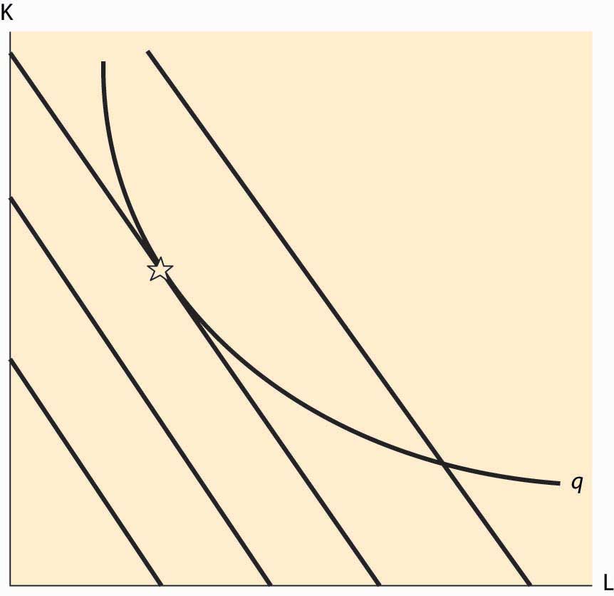
Figure 9.5 Tangency and Isoquants

There are circumstances where the cost-minimization feature of profit maximization can be used, and this is especially true when a graphical approach is taken. The graphical approach to profit maximization is illustrated in Figure 9.5 "Tangency and Isoquants". The curve represents an isoquant, which holds constant the output. The straight lines represent isocostLine that holds constant the expenditure on inputs. lines, which hold constant the expenditure on inputs. Isocost lines solve the problem rK + wL = constant and thus have slope Isocost lines are necessarily parallel—they have the same slope. Moreover, the cost associated with an isocost line rises the farther northeast we go in the graph, or the farther away from the origin.
What point on an isoquant minimizes total cost? The answer is the point associated with the lowest (most southwest) isocost that intersects the isoquant. This point will be tangent to the isoquant and is denoted by a star. At any lower cost, it isn’t possible to produce the desired quantity. At any higher cost, it is possible to lower cost and still produce the quantity.
The fact that cost minimization requires a tangency between the isoquant and the isocost has a useful interpretation. The slope of the isocost is minus the ratio of input prices. The slope of the isoquant measures the substitutability of the inputs in producing the output. Economists call this slope the marginal rate of technical substitutionThe amount of one input needed to make up for a decrease in another input while holding output constant., which is the amount of one input needed to make up for a decrease in another input while holding output constant. Thus, one feature of cost minimization is that the input price ratio equals the marginal rate of technical substitution.