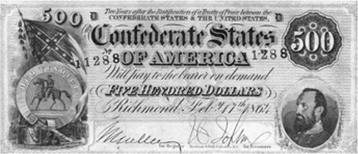
Many people purchase durable goods as investments, including Porsche Speedsters (see Figure 11.4 "The Porsche Speedster"), Tiffany lamps, antique telephones, postage stamps and coins, baseball cards, original Barbie dolls, antique credenzas, autographs, original rayon Hawaiian shirts, old postcards, political campaign buttons, old clocks, and even Pez dispensers. How is the value of, say, a 1961 Porsche Speedster or a $500 bill from the Confederacy, which currently sells for over $500, determined?
The theory of resource prices can be adapted to cover these items, which are in fixed supply. There are four major differences that are relevant. First, using the item doesn’t consume it: The goods are durable. I can own an “I Like Ike” campaign button for years, and then sell the same button. Second, these items may depreciate. Cars wear out even when they aren’t driven, and the brilliant color of Pez dispensers fades. Every time that a standard 27.5-pound gold bar, like the kind in the Fort Knox depository, is moved, approximately $5 in gold wears off the bar. Third, the goods may cost something to store. Fourth, the population grows, and some of the potential buyers are not yet born.
Figure 11.4 The Porsche Speedster

To understand the determinants of the prices of collectibles, it is necessary to create a major simplification to perform the analysis in continuous time. Let t, ranging from zero to infinity, be the continuous-time variable. If the good depreciates at rate δ, and q0 is the amount available at time 0, the quantity available at time t is .
For simplicity, assume that there is constant elasticity of demand ε. If g is the population growth rate, the quantity demanded, for any price p, is given by for a constant a that represents the demand at time 0. This represents demand for the good for direct use, but neglects the investment value of the good—the fact that the good can be resold for a higher price later. In other words, xd captures the demand for looking at Pez dispensers or driving Porsche Speedsters, but does not incorporate the value of being able to resell these items.
The demand equation can be used to generate the lowest use value to a person owning the good at time t. That marginal use value v arises from the equality of supply and demand:
or
Thus, the use value to the marginal owner of the good at time t satisfies
An important aspect of this development is that the value to the owner is found without reference to the price of the good. The reason this calculation is possible is that the individuals with high values will own the good, and the number of goods and the values of people are assumptions of the theory. Essentially, we already know that the price will ration the good to the individuals with high values, so computing the lowest value individual who holds a good at time t is a straightforward “supply equals demand” calculation. Two factors increase the marginal value to the owner—there are fewer units available because of depreciation, and there are more high-value people demanding them because of population growth. Together, these factors make the marginal use value grow at the rate
Assume that s is the cost of storage per unit of time and per unit of the good, so that storing x units for a period of length Δ costs sxΔ. This is about the simplest possible storage cost technology.
The final assumption we make is that all potential buyers use a common discount rate r, so that the discount of money or value received Δ units of time in the future is e-rΔ. It is worth a brief digression to explain why it is sensible to assume a common discount rate, when it is evident that many people have different discount rates. Different discount rates induce gains from trade in borrowing and lending, and create an incentive to have banks. While banking is an interesting topic to study, this section is concerned with collectibles, not banks. If we have different discount factors, then we must also introduce banks, which would complicate the model substantially. Otherwise, we would intermingle the theory of banking and the theory of collectibles. It is probably a good idea to develop a joint theory of banking and collectibles, given the investment potential of collectibles, but it is better to start with the pure theory of either one before developing the joint theory.
Consider a person who values the collectible at v. Is it a good thing for this person to own a unit of the good at time t? Let p be the function that gives the price across time, so that p(t) is the price at time t. Buying the good at time t and then selling what remains (recall that the good depreciates at rate δ) at time t + Δ gives a net value of
For the marginal person—that is, the person who is just indifferent to buying or not buying at time t—this must be zero at every moment in time, for Δ = 0. If v represents the value to a marginal buyer (indifferent to holding or selling) holding the good at time t, then this expression should come out to be zero. Thus, dividing by Δ,
Recall that the marginal value is , which gives The general solution to this differential equation is
It turns out that this equation only makes sense if for otherwise the present value of the marginal value goes to infinity, so there is no possible finite initial price. Provided that demand is elastic and discounting is larger than growth rates (which is an implication of equilibrium in the credit market), this condition will be met.
What is the initial price? It must be the case that the present value of the price is finite, for otherwise the good would always be a good investment for everyone at time 0, using the “buy and hold for resale” strategy. That is,
This condition implies that and thus
This equation may take on two different forms. First, it may be solvable for a nonnegative price, which happens if
Second, it may require destruction of some of the endowment of the good. Destruction must happen if the quantity of the good q0 at time 0 satisfies
In this case, there is too much of the good, and an amount must be destroyed to make the initial price zero. Since the initial price is zero, the good is valueless at time zero, and destruction of the good makes sense—at the current quantity, the good is too costly to store for future profits. Enough is destroyed to ensure indifference between holding the good as a collectible and destroying it. Consider, for example, the $500 Confederate bill shown in Figure 11.5 "$500 Confederate States bill". Many of these bills were destroyed at the end of the U.S. Civil War, when the currency became valueless and was burned as a source of heat. Now, an uncirculated version retails for $900.
Figure 11.5 $500 Confederate States bill

The amount of the good that must be destroyed is such that the initial price is zero. As q0 is the initial (predestruction) quantity, the amount at time zero after the destruction is the quantity q(0) satisfying
Given this construction, we have that
where either q(0) = q0 and p(0) ≥ 0, or q(0) < q0 and p(0) = 0.
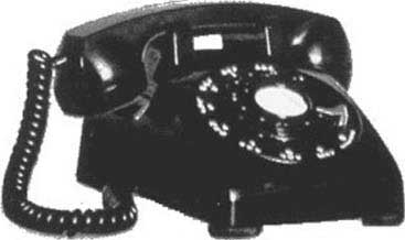
Destruction of a portion of the stock of a collectible, followed by price increases, is actually a quite common phenomenon. In particular, consider the “Model 500” telephone by Western Electric illustrated in Figure 11.6 "Western Electric Model 500 telephone". This ubiquitous classic phone was retired as the United States switched to tone dialing and push-button phones in the 1970s, and millions of phones—perhaps over 100 million—wound up in landfills. Now the phone is a collectible, and rotary phone enthusiasts work to keep them operational.
Figure 11.6 Western Electric Model 500 telephone

The solution for p(0) dramatically simplifies the expression for p(t):
This formula enables one to compare different collectibles. The first insight is that storage costs enter linearly into prices, so that growth rates are approximately unaffected by storage costs. The fact that gold is easy to store—while stamps and art require control of humidity and temperature in order to preserve value, and are hence more expensive to store—affects the level of prices but not the growth rate. However, depreciation and the growth of population affect the growth rate, and they do so in combination with the demand elasticity. With more elastic demand, prices grow more slowly and start at a lower level.