Chapter 11 Investment

11.1 Present Value

The promise of $1 in the future is not worth $1 today. There are a variety of reasons why a promise of future payments is not worth the face value today, some of which involve risk that the money may not be paid. Let’s set aside such risk for the moment. Even when the future payment is perceived to occur with negligible risk, most people prefer $1 today to $1 payable a year hence. One way to express this is by the present valueValue in today’s dollars of a stream of future payments.: The value today of a future payment of a dollar is less than a dollar. From a present value perspective, future payments are discountedThe practice of adjusting a sequence of payments to account for the interest these payments would earn in financial markets..

From an individual perspective, one reason that one should value a future payment less than a current payment is due to arbitrageBuying and reselling to make a profit..Arbitrage is the process of buying and selling in such a way as to make a profit. For example, if wheat is selling for $3 per bushel in New York but $2.50 per bushel in Chicago, one can buy in Chicago and sell in New York, profiting by $0.50 per bushel minus any transaction and transportation costs. Such arbitrage tends to force prices to differ by no more than transaction costs. When these transaction costs are small, as with gold, prices will be about the same worldwide. Suppose you are going to need $10,000 one year from now to put a down payment on a house. One way of producing $10,000 is to buy a government bond that pays $10,000 a year from now. What will that bond cost you? At current interest rates, a secure bondEconomists tend to consider U.S. federal government securities secure, because the probability of such a default is very, very low. will cost around $9,700. This means that no one should be willing to pay $10,000 for a future payment of $10,000 because, instead, one can have the future $10,000 by buying the bond, and will have $300 left over to spend on cappuccinos or economics textbooks. In other words, if you will pay $10,000 for a secure promise to repay the $10,000 a year hence, then I can make a successful business by selling you the secure promise for $10,000 and pocketing $300.

This arbitrage consideration also suggests how to value future payments: discount them by the relevant interest rate.

Example (Auto loan): You are buying a $20,000 car, and you are offered the choice to pay it all today in cash, or to pay $21,000 in one year. Should you pay cash (assuming you have that much in cash) or take the loan? The loan is at a 5% annual interest rate because the repayment is 5% higher than the loan amount. This is a good deal for you if your alternative is to borrow money at a higher interest rate; for example, on (most) credit cards. It is also a good deal if you have savings that pay more than 5%—if buying the car with cash entails cashing in a certificate of deposit that pays more than 5%, then you would be losing the difference. If, on the other hand, you are currently saving money that pays less than 5% interest, paying off the car is a better deal.

The formula for present value is to discount by the amount of interest. Let’s denote the interest rate for the next year as r₁, the second year’s rate as r₂, and so on. In this notation, $1 invested would pay $(1 + r₁) next year, or $(1 + r₁) × (1 + r₂) after 2 years, or $(1 + r₁) × (1 + r₂) × (1 + r₃) after 3 years. That is, r_i is the interest rate that determines the value, at the end of year i, of $1 invested at the start of year i. Then if we obtain a stream of payments A₀ immediately, A₁ at the end of year one, A₂ at the end of year two, and so on, the present value of that stream is

$$PV=A_0+\frac{A_1}{1+r_1}+\frac{A_2}{(1+r_1)(1+r_2)}+\frac{A_2}{(1+r_1)(1+r_2)(1+r_3)}+\mathrm{\dots }$$

Example (Consolidated annuities or consolsBonds that pay a fixed amount in perpetuity (forever).): What is the value of $1 paid at the end of each year forever, with a fixed interest rate r? Suppose the value is v. ThenThis development uses the formula that, for -1 < a < 1, $\frac{1}{1-a}=1+a+a^2+$ …, which is readily verified. Note that this formula involves an infinite series.

$$v=\frac{1}{1+r}+\frac{1}{{(1+r)}^2}+\frac{1}{{(1+r)}^3}+\mathrm{\dots }=\frac{1}{1-\frac{1}{1+r}}-1=\frac{1}{r}.$$

At a 5% interest rate, $1 million per year paid forever is worth $20 million today. Bonds that pay a fixed amount every year forever are known as consols; no current government issues consols.

Example (Mortgages): Again, fix an interest rate r, but this time let r be the monthly interest rate. A mortgage implies a fixed payment per month for a large number of months (e.g., 360 for a 30-year mortgage). What is the present value of these payments over n months? A simple way to compute this is to use the consol value, because

$$M=\frac{1}{1+r}+\frac{1}{{(1+r)}^2}+\frac{1}{{(1+r)}^3}+\mathrm{\dots }+\frac{1}{{(1+r)}^n}=\frac{1}{r}-\frac{1}{{(1+r)}^{n+1}}-\frac{1}{{(1+r)}^{n+2}}-\frac{1}{{(1+r)}^{n+3}}-\mathrm{\dots }$$ $$=\frac{1}{r}-\frac{1}{{(1+r)}^n}\left(\frac{1}{(1+r)}+\frac{1}{{(1+r)}^2}+\frac{1}{{(1+r)}^3}+\mathrm{\dots }\right)$$ $$=\frac{1}{r}-\frac{1}{{(1+r)}^n}\frac{1}{r}=\frac{1}{r}\left(1-\frac{1}{{(1+r)}^n}\right).$$

Thus, at a monthly interest rate of 0.5%, paying $1 per month for 360 months produces a present value M of $\frac{1}{0.005}\left(1-\frac{1}{{(1.005)}^{360}}\right)=\$166.79$ . Therefore, to borrow $100,000, one would have to pay $\frac{\$100,000}{\$166.79}=\text{\$599}\text{.55}$ per month. It is important to remember that a different loan amount just changes the scale: Borrowing $150,000 requires a payment of $\frac{\$150,000}{\$166.79}=\text{\$899}\text{.33}$ per month, because $1 per month generates $166.79 in present value.

Example (Simple and compound interest): In the days before calculators, it was a challenge to actually solve interest-rate formulas, so certain simplifications were made. One of these was simple interestAn approximate interest rate that is calculated by dividing the annual interest rate by the number of periods in one year., which meant that daily or monthly rates were translated into annual rates by incorrect formulas. For example, with an annual rate of 5%, the simple interest daily rate is $\frac{5\%}{365}=0.07692\%\text{.}$ The fact that this is incorrect can be seen from the calculation ${\left(1+\frac{.05}{365}\right)}^{365}=1.051267\%\text{,}$ which is the compound interestThe correct rate of interest that is calculated by adding together the cumulative interest payments earned during one year. calculation. Simple interest increases the annual rate, so it benefits lenders and harms borrowers. (Consequently, banks advertise the accurate annual rate on savings accounts—when consumers like the number to be larger—but not on mortgages, although banks are required by law to disclose, but not to advertise widely, actual annual interest rates on mortgages.)

Example (Obligatory lottery): You win the lottery, and the paper reports that you’ve won $20 million. You’re going to be paid $20 million, but is it worth $20 million? In fact, you get $1 million per year for 20 years. However, in contrast to our formula, you get the first million right off the bat, so the value is

$$PV=1+\frac{1}{1+r}+\frac{1}{{(1+r)}^2}+\frac{1}{{(1+r)}^3}+\mathrm{\dots }+\frac{1}{{(1+r)}^{19}}=1+\frac{1}{r}\left(1-\frac{1}{{(1+r)}^{19}}\right).$$

Table 11.1 "Present value of $20 million" computes the present value of our $20 million dollar lottery, listing the results in thousands of dollars, at various interest rates. At 10% interest, the value of the lottery is less than half the “number of dollars” paid; and even at 5%, the value of the stream of payments is 65% of the face value.

The lottery example shows that interest rates have a dramatic impact on the value of payments made in the distant future. Present value analysis is the number one tool used in MBA programs, where it is known as net present value, or NPVThe present value of a stream of net payments., analysis. It is accurate to say that the majority of corporate investment decisions are guided by an NPV analysis.

Example (Bond prices): A standard Treasury billA bond that has a fixed redemption value. has a fixed future value. For example, it may pay $10,000 in one year. It is sold at a discount off the face value, so that a one-year, $10,000 bond might sell for $9,615.39, producing a 4% interest rate. To compute the effective interest rate r, the formula relating the future value FV, the number of years n, and the price is

$${\left(1+r\right)}^n=\frac{FV}{\text{Price}}$$

or

$$r={\left(\frac{FV}{\text{Price}}\right)}^{\raisebox{1ex}{$1$}\!\left/ \!\raisebox{-1ex}{$n$}\right.}-1.$$

We can see from either formula that Treasury bill prices move inversely to interest rates—an increase in interest rates reduces Treasury prices. Bonds are a bit more complicated. Bonds pay a fixed interest rate set at the time of issue during the life of the bond, generally collected semiannually, and the face value is paid at the end of the term. These bonds were often sold on long terms, as much as 30 years. Thus, a three-year, $10,000 bond at 5% with semiannual payments would pay $250 at the end of each half year for 3 years, and pay $10,000 at the end of the 3 years. The net present value, with an annual interest rate r, is

$$NPV=\frac{\$250}{{\left(1+r\right)}^{\raisebox{1ex}{$1$}\!\left/ \!\raisebox{-1ex}{$2$}\right.}}+\frac{\$250}{{\left(1+r\right)}^1}+\frac{\$250}{{\left(1+r\right)}^{\raisebox{1ex}{$3$}\!\left/ \!\raisebox{-1ex}{$2$}\right.}}+\frac{\$250}{{\left(1+r\right)}^2}+\frac{\$250}{{\left(1+r\right)}^{\raisebox{1ex}{$5$}\!\left/ \!\raisebox{-1ex}{$2$}\right.}}+\frac{\$250}{{\left(1+r\right)}^3}+\frac{\$10000}{{\left(1+r\right)}^3}.$$

The net present value will be the price of the bond. Initially, the price of the bond should be the face value, since the interest rate is set as a market rate. The U.S. Treasury quit issuing such bonds in 2001, replacing them with bonds in which the face value is paid and then interest is paid semiannually.

11.2 Investment

A simple investment project requires an investment, I, followed by a return over time. If you dig a mine, drill an oil well, build an apartment building or a factory, or buy a share of stock, you spend money now, hoping to earn a return in the future. We will set aside the very important issue of risk until the next subsection, and ask how one makes the decision to invest.

The NPV approach involves assigning a rate of return r that is reasonable for the specific project and then computing the corresponding present value of the expected stream of payments. Since the investment is initially expended, it is counted as negative revenue. This yields an expression that looks like

$$NPV=-I+\frac{R_1}{1+r}+\frac{R_2}{{(1+r)}^2}+\frac{R_3}{{(1+r)}^3}+\mathrm{\dots .}$$

where R₁ represents first-year revenues, R₂ represents second-year revenues, and so on.The most common approach treats revenues within a year as if they are received at the midpoint, and then discounts appropriately for that mid-year point. The present discussion abstracts from this practice. The investment is then made when NPV is positive—because this would add to the net value of the firm.

Carrying out an NPV analysis requires two things. First, investment and revenues must be estimated. This is challenging, especially for new products where there is no direct way of estimating demand, or with uncertain outcomes like oil wells or technological research.The building of the famed Sydney Opera House, which looks like billowing sails over Sydney Harbor in Australia, was estimated to cost $7 million and actually cost $105 million. A portion of the cost overrun was due to the fact that the original design neglected to install air conditioning. When this oversight was discovered, it was too late to install a standard unit, which would interfere with the excellent acoustics, so instead an ice hockey floor was installed as a means of cooling the building. Second, an appropriate rate of return must be identified. The rate of return is difficult to estimate, mostly because of the risk associated with the investment payoffs. Another difficulty is recognizing that project managers have an incentive to inflate the payoffs and minimize the costs to make the project appear more attractive to upper management. In addition, most corporate investment is financed through retained earnings, so that a company that undertakes one investment is unable to make other investments, so the interest rate used to evaluate the investment should account for opportunity cost of corporate funds. As a result of these factors, interest rates of 15%–20% are common for evaluating the NPV of projects of major corporations.

Example (Silver mine): A company is considering developing a silver mine in Mexico. The company estimates that developing the mine requires building roads and opening a large hole in the ground, which would cost $4 million per year for 4 years, during which time the mines generates zero revenue. Starting in year 5, the expenses would fall to $2 million per year, and $6 million in net revenue would accrue from the silver that is mined for the next 40 years. If the company cost of funds is 18%, should it develop the mine?

The earnings from the mine are calculated in the table below. First, the NPV of the investment phase during years 0, 1, 2, and 3 is

$$NPV=-4+\frac{-4}{1.18}+\frac{-4}{{(1.18)}^2}+\frac{-4}{{(1.18)}^3}=-\mathrm{12.697.}$$

A dollar earned in each of years 4 through 43 has a present value of

$$\frac{1}{{(1+r)}^4}+\frac{1}{{(1+r)}^5}+\frac{1}{{(1+r)}^6}+\mathrm{\dots }+\frac{1}{{(1+r)}^{43}}=\frac{1}{{(1+r)}^3}\times \frac{1}{r}\left(1-\frac{1}{{(1+r)}^{40}}\right)=\mathrm{13.377.}$$

The mine is just profitable at 18%, in spite of the fact that its $4 million payments are made in 4 years, after which point $4 million in revenue is earned for 40 years. The problem in the economics of mining is that 18% makes the future revenue have quite modest present values.

There are other approaches for deciding to take an investment. In particular, the internal rate of return (IRR)Method of analyzing an investment that solves the equation NPV = 0 for the interest rate. approach solves the equation NPV = 0 for the interest rate. Then the project is undertaken if the rate of return is sufficiently high. This approach is flawed because the equation may have more than one solution—or no solutions—and the right thing to do in these events is not transparent. Indeed, the IRR approach gets the profit-maximizing answer only if it agrees with NPV. A second approach is the payback period, which asks calculates the number of years a project must be run before profitability is reached. The problem with the payback period is deciding between projects—if I can only choose one of two projects, the one with the higher NPV makes the most money for the company. The one with the faster payback may make a quite small amount of money very quickly, but it isn’t apparent that this is a good choice. When a company is in risk of bankruptcy, a short payback period might be valuable, although this would ordinarily be handled by employing a higher interest rate in an NPV analysis. NPV does a good job when the question is whether or not to undertake a project, and it does better than other approaches to investment decisions. For this reason, NPV has become the most common approach to investment decisions. Indeed, NPV analysis is more common than all other approaches combined. NPV does a poor job, however, when the question is whether to undertake a project or to delay the project. That is, NPV answers “yes or no” to investment, but when the choice is “yes or wait,” NPV requires an amendment.

11.3 Investment Under Uncertainty

Risk has a cost, and people and corporations buy insurance against financial risk.For example, NBC spent $6 million to buy an insurance policy against U.S. nonparticipation in the 1980 Moscow Summer Olympic Games—and the United States didn’t participate (because of the Soviet invasion of Afghanistan)—and NBC was paid $94 million from the policy. The standard approach to investment under uncertainty is to compute an NPV, using a “risk-adjusted” interest rate to discount the expected values received over time. The interest rate is increased or lowered depending on how risky the project is.

For example, consider a project like oil exploration. The risks are enormous. Half of all underwater tracts in the Gulf Coast near Louisiana and Texas that are leased are never drilled, because they turn out to be a bad bet. Half of all the tracts that are drilled are dry. Hence, three quarters of the tracts that are sold produce zero or negative revenue. To see how the economics of such a risky investment might be developed, suppose that the relevant rate of return for such investments is 18%. Suppose further that the tract can be leased for $500,000 and the initial exploration costs $1 million. If the tract has oil (with a 25% probability), it produces $1 million per year for 20 years and then runs dry. This gives an expected revenue of $250,000 per year. To compute the expected net present value, we first compute the returns:

At 18%, the investment is a loss—the risk is too great given the average returns.

A very important consideration for investment under uncertainty is the choice of interest rate. It is crucial to understand that the interest rate is specific to the project and not to the investor. This is perhaps the most important insight of corporate finance generally: The interest rate should adjust for the risk associated with the project and not for the investor. For example, suppose hamburger retailer McDonald’s is considering investing in a cattle ranch in Peru. McDonald’s is overall a very low-risk firm, but this particular project is quite risky because of local conditions. McDonald’s still needs to adjust for the market value of the risk it is undertaking, and that value is a function of the project risk, not the risk of McDonald’s other investments.

This basic insight of corporate financeThe study of funding of operations of companies. (the study of funding of operations of companies)—the appropriate interest rate is determined by the project, not by the investor—is counterintuitive to most of us because it doesn’t apply to our personal circumstances. For individuals, the cost of borrowing money is mostly a function of our own personal circumstances, and thus the decision of whether to pay cash for a car or borrow the money is not so much a function of the car that is being purchased but of the wealth of the borrower. Even so, personal investors borrow money at distinct interest rates. Mortgage rates on houses are lower than interest rates on automobiles, and interest rates on automobiles are lower than on credit cards. This is because the “project” of buying a house has less risk associated with it: The percentage loss to the lender in the event of borrower default is lower on a house than on a car. Credit cards carry the highest interest rates because they are unsecured by any asset.

One way of understanding why the interest rate is project-specific, but not investor-specific, is to think about undertaking the project by creating a separate firm to make the investment. The creation of subsidiary units is a common strategy, in fact. This subsidiary firm created to operate a project has a value equal to the NPV of the project using the interest rate specific to the subsidiary, which is the interest rate for the project, independent of the parent. For the parent company, owning such a firm is a good thing if the firm has positive value, but not otherwise.It may seem that synergies between parent and subsidiary are being neglected here, but synergies should be accounted for at the time they produce value—that is, as part of the stream of revenues of the subsidiary.

Investments in oil are subject to another kind of uncertainty: price risk. The price of oil fluctuates. Moreover, oil pumped and sold today is not available for the future. Should you develop and pump the oil you have today, or should you hold out and sell in the future? This question, known as the option value of investment, is generally somewhat challenging and arcane, but a simple example provides a useful insight. An optionThe right to buy or sell at a price determined in advance. is the right to buy or sell at a price determined in advance.

To develop this example, let’s set aside some extraneous issues first. Consider a very simple investment, in which either C is invested or not.This theory is developed in striking generality by Avinash Dixit and Robert Pindyck, Investment Under Uncertainty, Princeton University Press, 1994. If C is invested, a value V is generated. The cost C is a constant; it could correspond to drilling or exploration costs or, in the case of a stock option, the strike priceThe amount one pays to obtain a share of stock. of the option, which is the amount one pays to obtain the share of stock. The value V, in contrast, varies from time to time in a random fashion. To simplify the analysis, we assume that V is uniformly distributed on the interval [0, 1], so that the probability of V falling in an interval [a, b] is (b – a) if 0 ≤a ≤ b ≤ 1. The option only has value if C < 1, which we assume for the rest of this section.

The first thing to note is that the optimal rule to make the investment is a cutoff value—that is, to set a level V₀ and exercise the option if, and only if, V ≥ V₀. This is because—if you are willing to exercise the option and generate value V—you should be willing to exercise the option and obtain even more value. The NPV rule simply says V₀ = C; that is, invest whenever it is profitable. The purpose of the example developed below is to provide some insight into how far wrong the NPV rule will be when option values are potentially significant.

Now consider the value of option to invest, given that the investment rule V ≥ V₀ is followed. Call this option value J(V₀). If the realized value V exceeds V₀, one obtains V – C. Otherwise, one delays the investment, producing a discounted level of the same value. This logic says,

$$J(V_0)=(1-V_0)\left(\frac{1+V_0}{2}-C\right)+V_0\left(\frac{1}{1+r}J(V_0)\right).$$

This expression for J(V₀) is explained as follows. First, the hypothesized distribution of V is uniform on [0, 1]. Consequently, the value of V will exceed V₀ with probability 1 – V₀. In this event, the expected value of V is the midpoint of the interval [V₀, 1], which is ½(V₀ + 1). The value ½(V₀ + 1) – C is the average payoff from the strategy of investing whenever V ≥ V₀, which is obtained with probability 1 – V₀. Second, with probability V₀, the value falls below the cutoff level V₀. In this case, no investment is made and, instead, we wait until the next period. The expected profits of the next period are J(V₀), and these profits are discounted in the standard way.

The expression for J is straightforward to solve:

$$J(V_0)=\frac{(1-V_0)\left(\frac{1+V_0}{2}-C\right)}{1-\frac{V_0}{1+r}}$$

Rudimentary calculus shows

$$J^{\prime }(V_0)=\frac{1+2rC+V_0^2-2(1+r)V_0}{2(1+r){\left(1-\frac{V_0}{1+r}\right)}^2}.$$

First, note that $J^{\prime }(C)>0$ and $J^{\prime }(1)<0\text{,}$ which together imply the existence of a maximum at a value V₀ between C and 1, satisfying $J^{\prime }(V_0)=0\text{.}$ Second, the solution occurs at

$$V_0=(1+r)-\sqrt{{(1+r)}^2-(1+2rC)}=(1+r)-\sqrt{r^2+2r(1-C)}.$$

The positive root of the quadratic has V₀ > 1, which entails never investing, and hence is not a maximum. The profit-maximizing investment strategy is to invest whenever the value exceeds V₀ given by the negative root in the formula. There are a couple of notable features about this solution. First, at r = 0, V₀ = 1. This is because r = 0 corresponds to no discounting, so there is no loss in holding out for the highest possible value. Second, as r → ∞, V₀ → C. As r → ∞, the future is valueless, so it is worth investing if the return is anything over costs. These are not surprising findings, but rather quite the opposite: They should hold in any reasonable formulation of such an investment strategy. Moreover, they show that the NPV rule, which requires V₀ = C, is correct only if the future is valueless.

How does this solution behave? The solution is plotted as a function of r, for C = 0, 0.25, and 0.5, in Figure 11.1 "Investment strike price given interest rate ".

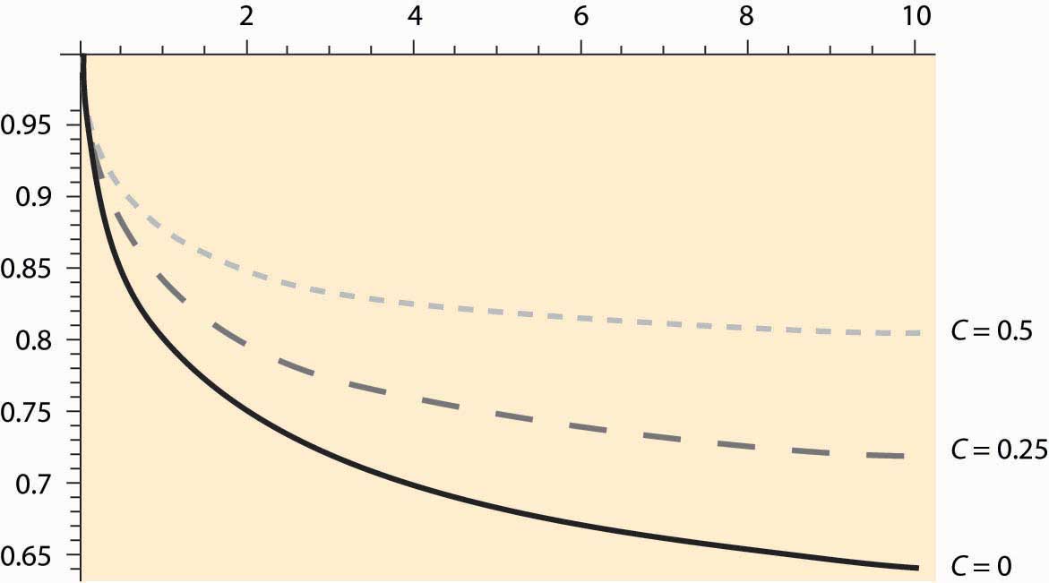
The horizontal axis represents interest rates, so this figure shows very high interest rates by current standards, up to 200%. Even so, V₀ remains substantially above C. That is, even when the future has very little value, because two-thirds of the value is destroyed by discounting each period, the optimal strategy deviates significantly from the NPV strategy. Figure 11.2 "Investment strike price given interest rate " shows a close-up of this graph for a more reasonable range of interest rates, for interest rates of 0%–10%.

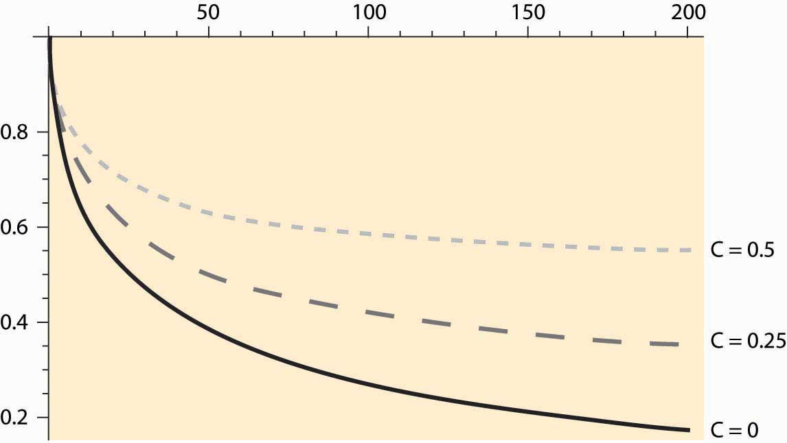
Figure 11.2 "Investment strike price given interest rate " shows the cutoff values of investment for three values of C, the cost of the investment. These three values are 0 (lowest curve), 0.25 (the middle, dashed curve), and 0.5 (the highest, dotted line). Consider the lowest curve, with C = 0. The NPV of this project is always positive—there are no costs, and revenues are positive. Nevertheless, because the investment can only be made once, it pays to hold out for a higher level of payoff; indeed, for 65% or more of the maximum payoff. The economics at an interest rate of 10% is as follows. By waiting, there is a 65% chance that 10% of the potential value of the investment is lost. However, there is a 35% chance of an even higher value. The optimum value of V₀ trades these considerations off against each other.

For C = 0.25, at 10% the cutoff value for taking an investment is 0.7, nearly three times the actual cost of the investment. Indeed, the cutoff value incorporates two separate costs: the actual expenditure on the investment C and the lost opportunity to invest in the future. The latter cost is much larger than the expenditure on the investment in many circumstances and, in this example, can be quantitatively much larger than the actual expenditure on the investment.

Some investments can be replicated. There are over 13,000 McDonald’s restaurants in the United States, and building another one doesn’t foreclose building even more. For such investments, NPV analysis gets the right answer, provided that appropriate interest rates and expectations are used. Other investments are difficult to replicate or logically impossible to replicate—having pumped and sold the oil from a tract, that tract is now dry. For such investments, NPV is consistently wrong because it neglects the value of the option to delay the investment. A correct analysis adds a lost value for the option to delay the cost of the investment—a value that can be quantitatively large—as we have seen.

Example: When should you refinance a mortgage? Suppose you are paying 10% interest on a $100,000 mortgage, and it costs $5,000 to refinance; but refinancing permits you to lock in a lower interest rate, and hence pay less. When is it a good idea? To answer this question, we assume that the $5,000 cost of refinancing is built into the loan so that, in essence, you borrow $105,000 at a lower interest rate when you refinance. This is actually the most common method of refinancing a mortgage.

To simplify the calculations, we will consider a mortgage that is never paid off; that is, one pays the same amount per year forever. If the mortgage isn’t refinanced, one pays 10% of the $100,000 face value of the mortgage each year, or $10,000 per year. If one refinances at interest rate r, one pays r × $105,000 per year, so the NPV of refinancing is

NPV = $10,000 – r × $105,000.

Thus, NPV is positive whenever $r<\frac{10}{105}=9.52\%\text{.}$

Should you refinance when the interest rate drops to this level? No. At this level, you would exactly break even, but you would also be carrying a $105,000 mortgage rather than a $100,000 mortgage, making it harder to benefit from any further interest-rate decreases. The only circumstance in which refinancing at 9.52% is sensible is if interest rates can’t possibly fall further.

When should you refinance? That depends on the nature and magnitude of the randomness governing interest rates, preferences over money today versus money in the future, and attitudes to risk. The model developed in this section is not a good guide to answering this question, primarily because the interest rates are strongly correlated over time. However, an approximate guide to implementing the option theory of investment is to seek an NPV of twice the investment, which would translate into a refinance point of around 8.5%.

11.4 Resource Extraction

For the past 60 years, the world has been “running out of oil.” There are news stories about the end of the reserves being only 10, 15, or 20 years away. The tone of these stories is that, at this time, we will run out of oil completely and prices will be extraordinarily high. Industry studies counter that more oil continues to be found and that the world is in no danger of running out of oil.

If you believe that the world will run out of oil, what should you do? You should buy and hold. That is, if the price of oil in 20 years is going to be $1,000 per barrel, then you can buy oil at $40 per barrel, hold it for 20 years, and sell it at $1,000 per barrel. The rate of return from this behavior is the solution to ${(1+r)}^{20}=\frac{1000}{40}\text{.}$

This equation solves for r = 17.46%, which represents a healthy rate of return on investment. This substitution is part of a general conclusion known as the Ramsey ruleFor resources in fixed supply, prices rise at the interest rate.:The solution to this problem is known as Ramsey pricing, after the discoverer Frank Ramsey (1903–1930). For resources in fixed supply, prices rise at the interest rate. With a resource in fixed supply, owners of the resource will sell at the point maximizing the present value of the resource. Even if they do not, others can buy the resource at the low present value of price point, resell at the high present value, and make money.

The Ramsey rule implies that prices of resources in fixed supply rise at the interest rate. An example of the Ramsey rule in action concerns commodities that are temporarily fixed in supply, such as grains after the harvest. During the period between harvests, these products rise in price on average at the interest rate, where the interest rate includes storage and insurance costs, as well as the cost of funds.

Example: Let time be t = 0, 1, … , and suppose the demand for a resource in fixed supply has constant elasticity: $p(Q)=a{Q}^{\raisebox{1ex}{$-1$}\!\left/ \!\raisebox{-1ex}{$\epsilon $}\right.}\text{.}$ Suppose that there is a total stock R of the resource, and the interest rate is fixed at r. What is the price and consumption of the resource at each time?

Solution: Let Qt represent the quantity consumed at time t. Then the arbitrage condition requires

$$a{Q}_0^{\raisebox{1ex}{$-1$}\!\left/ \!\raisebox{-1ex}{$\epsilon $}\right.}{(1+r)}^t=p(Q_0){(1+r)}^t=p(Q_t)=a{Q}_t^{\raisebox{1ex}{$-1$}\!\left/ \!\raisebox{-1ex}{$\epsilon $}\right.}\text{.}$$

Thus, $Q_t=Q_0{(1+r)}^{-t\epsilon }\text{.}$ Finally, the resource constraint implies

$$R=(Q_0+Q_1+Q_2+\mathrm{\dots })=Q_0\left(1+{(1+r)}^{-\epsilon }+{(1+r)}^{-2\epsilon }+\mathrm{\dots }\right)=\frac{Q_0}{1-{(1+r)}^{-\epsilon }}.$$

This solves for the initial consumption Q₀. Consumption in future periods declines geometrically, thanks to the constant elasticity assumption.

Market arbitrage ensures the availability of the resource in the future and drives up the price to ration the good. The world runs out slowly, and the price of a resource in fixed supply rises on average at the interest rate.

Resources like oil and minerals are ostensibly in fixed supply—there is only so much oil, gold, bauxite, or palladium in the earth. Markets, however, behave as if there is an unlimited supply, and with good reason. People are inventive and find substitutes. England’s wood shortage of 1651 didn’t result in England being cold permanently, nor was England limited to the wood it could grow as a source of heat. Instead, coal was discovered. The shortage of whale oil in the mid-19th century led to the development of oil resources as a replacement. If markets expect that price increases will lead to substitutes, then we rationally should use more today, trusting that technological developments will provide substitutes.Unlike oil and trees, whales were overfished and there was no mechanism for arbitraging them into the future—that is, no mechanism for capturing and saving whales for later use. This problem, known as the tragedy of the commons, results in too much use (Garett Hardin, Science, 1968, Tragedy of the Commons). Trees have also been overcut, most notably on Easter Island. Thus, while some believe that we are running out of oil, most investors are betting that we are not, and that energy will not be very expensive in the future—either because of continued discovery of oil or because of the creation of alternative energy sources. If you disagree, why not invest and take the bet? If you bet on future price increases, that will tend to increase the price today, encouraging conservation today, and increase the supply in the future.

11.5 A Time to Harvest

A tree grows slowly but is renewable, so the analysis of Section 11.4 "Resource Extraction" doesn’t help us to understand when it is most profitable to cut down the tree. Consider harvesting for pulp and paper use. In this case, the amount of wood chips is what matters to the profitability of cutting down the tree, and the biomass of the tree provides a direct indication of this. Suppose the biomass sells for a net price p, which has the costs of harvesting and replanting deducted from it, and the biomass of the tree is b(t) when the tree is t years old. It simplifies the analysis slightly to use continuous time discounting $e^{-\rho t}={\left(\frac{1}{1+r}\right)}^t\text{,}$ where$\rho =\log (1+r)\text{.}$

Consider the policy of cutting down trees when they are T years old. This induces a cutting cycle of length T. A brand new tree will produce a present value of profits of

$$e^{-\rho T}pb(T)+e^{-2\rho T}pb(T)+e^{-3\rho T}pb(T)+\dots =\frac{e^{-\rho T}pb(T)}{1-e^{-\rho T}}=\frac{pb(T)}{e^{\rho T}-1}\text{.}$$

This profit arises because the first cut occurs at time T, with discounting e^-ρT, and produces a net gain of pb(T). The process then starts over, with a second tree cut down at time 2T, and so on.

Profit maximization gives a first-order condition on the optimal cycle length T of

$$0=\frac{d}{dT}\frac{pb(T)}{e^{\rho T}-1}=\frac{p{b}^{\prime }(T)}{e^{\rho T}-1}-\frac{pb(T)\rho e^{\rho T}}{{\left(e^{\rho T}-1\right)}^2}$$

This can be rearranged to yield

$$\frac{b^{\prime }(T)}{b(T)}=\frac{\rho }{1-e^{-\rho T}}\text{.}$$

The left-hand side of this equation is the growth rate of the tree. The right-hand side is approximately the continuous-time discount factor, at least when T is large, as it tends to be for trees, which are usually on a 20- to 80-year cycle, depending on the species. This is the basis for a conclusion: Cut down the tree slightly before it is growing at the interest rate. The higher that interest rates are, the shorter the cycle for which the trees should be cut down.

The pulp and paper use of trees is special, because the tree is going to be ground up into wood chips. What happens when the object is to get boards from the tree, and larger boards sell for more? In particular, it is more profitable to get a 4 × 4 than two 2 × 4s. Doubling the diameter of the tree, which approximately raises the biomass by a factor of six to eight, more than increases the value of the timber by the increase in the biomass.

It turns out that our theory is already capable of handling this case. The only adaptation is a change in the interpretation of the function b. Now, rather than representing the biomass, b(t) must represent the value in boards of a tree that is t years old. (The parameter p may be set to one.) The only amendment to the rule for cutting down trees is as follows: The most profitable point in time to cut down the tree occurs slightly before the time when the value (in boards) of the tree is growing at the interest rate.

For example, lobsters become more valuable as they grow. The profit-maximizing time to harvest lobsters is governed by the same equation, where b(T) is the value of a lobster at age T. Prohibiting the harvest of lobsters under age T is a means of insuring the profit-maximizing capture of lobsters and preventing overfishing.

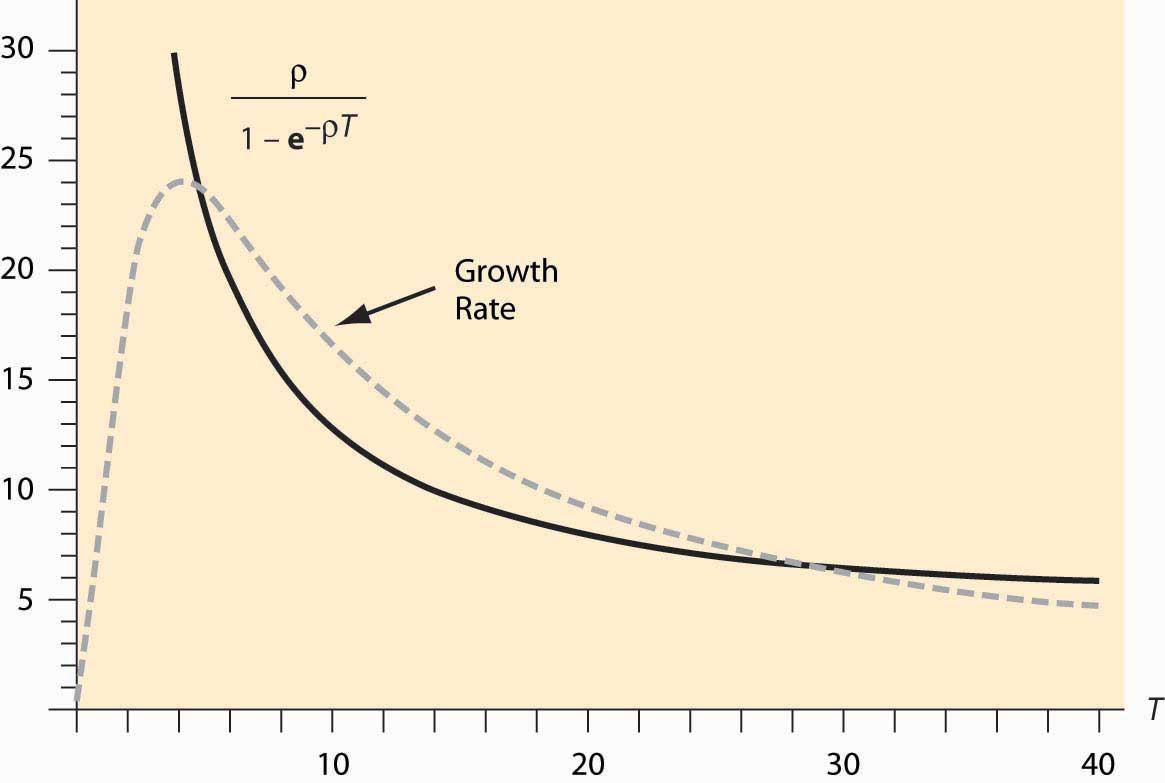
The implementation of the formula is illustrated in Figure 11.3 "Optimal solution for T". The dashed line represents the growth rate $\raisebox{1ex}{$b^{\prime }(T)$}\!\left/ \!\raisebox{-1ex}{$b(T)$}\right.\text{,}$ while the solid line represents the discount rate, which was set at 5%. Note that the best time to cut down the trees is when they are approximately 28.7 years old and, at that time, they are growing at 6.5%. Figure 11.3 "Optimal solution for T" also illustrates another feature of the optimization—there may be multiple solutions to the optimization problem, and the profit-maximizing solution involves $\raisebox{1ex}{$b^{\prime }(T)$}\!\left/ \!\raisebox{-1ex}{$b(T)$}\right.$ cutting $\frac{\rho }{1-e^{-\rho T}}$ from above.

The U.S. Department of the Interior is in charge of selling timber rights on federal lands. The department uses the policy of maximum sustainable yieldPolicy that maximizes the long-run average value of a sustainable resource. to determine the specific time that the tree is cut down. Maximum sustainable yield maximizes the long-run average value of the trees cut down; that is, it maximizes $\frac{b(T)}{T}\text{.}$

Maximum sustainable yield is actually a special case of the policies considered here, and arises for a discount factor of 0. It turns out (thanks to a formula known variously as l’Hôpital’s or l’Hospital’s Rule) that the $\underset{\rho \to 0}{\lim }\frac{\rho }{1-e^{-\rho T}}=\frac{1}{T}\text{.}$

Thus, the rule $\frac{b^{\prime }(T)}{b(T)}=\frac{\rho }{1-e^{-\rho T}}\to \frac{1}{T}$ as ρ → 0, and this is precisely the same rule that arises under maximum sustainable yield.

Thus, the Department of the Interior acts as if the interest rate is zero when it is not. The justification given is that the department is valuing future generations at the same level as current generations—that is, increasing the supply for future generations while slightly harming the current generation of buyers. The major consequence of the department’s policy of maximum sustainable yield is to force cutting of timber even when prices are low during recessions.

11.6 Collectibles

Many people purchase durable goods as investments, including Porsche Speedsters (see Figure 11.4 "The Porsche Speedster"), Tiffany lamps, antique telephones, postage stamps and coins, baseball cards, original Barbie dolls, antique credenzas, autographs, original rayon Hawaiian shirts, old postcards, political campaign buttons, old clocks, and even Pez dispensers. How is the value of, say, a 1961 Porsche Speedster or a $500 bill from the Confederacy, which currently sells for over $500, determined?

The theory of resource prices can be adapted to cover these items, which are in fixed supply. There are four major differences that are relevant. First, using the item doesn’t consume it: The goods are durable. I can own an “I Like Ike” campaign button for years, and then sell the same button. Second, these items may depreciate. Cars wear out even when they aren’t driven, and the brilliant color of Pez dispensers fades. Every time that a standard 27.5-pound gold bar, like the kind in the Fort Knox depository, is moved, approximately $5 in gold wears off the bar. Third, the goods may cost something to store. Fourth, the population grows, and some of the potential buyers are not yet born.

To understand the determinants of the prices of collectibles, it is necessary to create a major simplification to perform the analysis in continuous time. Let t, ranging from zero to infinity, be the continuous-time variable. If the good depreciates at rate δ, and q₀ is the amount available at time 0, the quantity available at time t is $q(t)=q_0{e}^{-\delta t}$ .

For simplicity, assume that there is constant elasticity of demand ε. If g is the population growth rate, the quantity demanded, for any price p, is given by $x_d(p,t)=a{e}^{gt}{p}^{-\epsilon }\text{,}$ for a constant a that represents the demand at time 0. This represents demand for the good for direct use, but neglects the investment value of the good—the fact that the good can be resold for a higher price later. In other words, xd captures the demand for looking at Pez dispensers or driving Porsche Speedsters, but does not incorporate the value of being able to resell these items.

The demand equation can be used to generate the lowest use value to a person owning the good at time t. That marginal use value v arises from the equality of supply and demand:

$$q_0{e}^{-\delta t}=q(t)=x_d(v,t)=a{e}^{gt}{v}^{-\epsilon }$$

or

$$v^{\epsilon }=\frac{a}{q_0}{e}^{(\delta +g)t}$$

Thus, the use value to the marginal owner of the good at time t satisfies $v={\left(\frac{a}{q_0}\right)}^{\raisebox{1ex}{$1$}\!\left/ \!\raisebox{-1ex}{$\epsilon $}\right.}{e}^{\frac{\delta +g}{\epsilon }t}\text{.}$

An important aspect of this development is that the value to the owner is found without reference to the price of the good. The reason this calculation is possible is that the individuals with high values will own the good, and the number of goods and the values of people are assumptions of the theory. Essentially, we already know that the price will ration the good to the individuals with high values, so computing the lowest value individual who holds a good at time t is a straightforward “supply equals demand” calculation. Two factors increase the marginal value to the owner—there are fewer units available because of depreciation, and there are more high-value people demanding them because of population growth. Together, these factors make the marginal use value grow at the rate $\frac{\delta +g}{\epsilon }\text{.}$

Assume that s is the cost of storage per unit of time and per unit of the good, so that storing x units for a period of length Δ costs sxΔ. This is about the simplest possible storage cost technology.

The final assumption we make is that all potential buyers use a common discount rate r, so that the discount of money or value received Δ units of time in the future is e^-rΔ. It is worth a brief digression to explain why it is sensible to assume a common discount rate, when it is evident that many people have different discount rates. Different discount rates induce gains from trade in borrowing and lending, and create an incentive to have banks. While banking is an interesting topic to study, this section is concerned with collectibles, not banks. If we have different discount factors, then we must also introduce banks, which would complicate the model substantially. Otherwise, we would intermingle the theory of banking and the theory of collectibles. It is probably a good idea to develop a joint theory of banking and collectibles, given the investment potential of collectibles, but it is better to start with the pure theory of either one before developing the joint theory.

Consider a person who values the collectible at v. Is it a good thing for this person to own a unit of the good at time t? Let p be the function that gives the price across time, so that p(t) is the price at time t. Buying the good at time t and then selling what remains (recall that the good depreciates at rate δ) at time t + Δ gives a net value of ${\displaystyle \underset{0}{\overset{\Delta }{\int }}{e}^{-ru}(v-s})du-p(t)+e^{-r\Delta }{e}^{-\delta \Delta }p(t+\Delta )\text{.}$

For the marginal person—that is, the person who is just indifferent to buying or not buying at time t—this must be zero at every moment in time, for Δ = 0. If v represents the value to a marginal buyer (indifferent to holding or selling) holding the good at time t, then this expression should come out to be zero. Thus, dividing by Δ,

$$0=\underset{\Delta \to 0}{\lim }\frac{1}{\Delta }{\displaystyle \underset{0}{\overset{\Delta }{\int }}{e}^{-ru}(v-s})du-\frac{p(t)}{\Delta }+\frac{e^{-(r+\delta )\Delta }p(t+\Delta )}{\Delta }$$ $=\underset{\Delta \to 0}{\lim }v-s+\frac{p(t+\Delta )-p(t)}{\Delta }-\frac{1-e^{-(r+\delta )\Delta }}{\Delta }p(t+\Delta )=v-s+p^{\prime }(t)-(r+\delta )p(t)\text{.}$

Recall that the marginal value is $v={\left(\frac{a}{q_0}\right)}^{\raisebox{1ex}{$1$}\!\left/ \!\raisebox{-1ex}{$\epsilon $}\right.}{e}^{\frac{\delta +g}{\epsilon }t}$ , which gives $p^{\prime }(t)=(r+\delta )p(t)+s-v=(r+\delta )p(t)+s-{\left(\frac{a}{q_0}\right)}^{\raisebox{1ex}{$1$}\!\left/ \!\raisebox{-1ex}{$\epsilon $}\right.}{e}^{\frac{\delta +g}{\epsilon }t}\text{.}$ The general solution to this differential equation is

$$p(t)=e^{(r+\delta )t}\left(p(0)+\frac{1-e^{-(r+\delta )t}}{(r+\delta )}s-{\left(\frac{a}{q_0}\right)}^{\raisebox{1ex}{$1$}\!\left/ \!\raisebox{-1ex}{$\epsilon $}\right.}\frac{1-e^{-\left(r+\delta -\frac{\delta +g}{\epsilon }\right)t}}{r+\delta -\frac{\delta +g}{\epsilon }}\right)\text{.}$$

It turns out that this equation only makes sense if $r+\delta -\frac{\delta +g}{\epsilon }>0\text{,}$ for otherwise the present value of the marginal value goes to infinity, so there is no possible finite initial price. Provided that demand is elastic and discounting is larger than growth rates (which is an implication of equilibrium in the credit market), this condition will be met.

What is the initial price? It must be the case that the present value of the price is finite, for otherwise the good would always be a good investment for everyone at time 0, using the “buy and hold for resale” strategy. That is,

$$\underset{t\to \infty }{\lim }{e}^{-rt}p(t)<\infty .$$

This condition implies that $\underset{t\to \infty }{\lim }{e}^{\delta t}\left(p(0)+\frac{1-e^{-(r+\delta )t}}{(r+\delta )}s-{\left(\frac{a}{q_0}\right)}^{\raisebox{1ex}{$1$}\!\left/ \!\raisebox{-1ex}{$\epsilon $}\right.}\frac{1-e^{-\left(r+\delta -\frac{\delta +g}{\epsilon }\right)t}}{r+\delta -\frac{\delta +g}{\epsilon }}\right)<\infty \text{,}$ and thus $p(0)+\frac{1}{(r+\delta )}s-{\left(\frac{a}{q_0}\right)}^{\raisebox{1ex}{$1$}\!\left/ \!\raisebox{-1ex}{$\epsilon $}\right.}\frac{1}{r+\delta -\frac{\delta +g}{\epsilon }}=0\text{.}$

This equation may take on two different forms. First, it may be solvable for a nonnegative price, which happens if

$$p(0)={\left(\frac{a}{q_0}\right)}^{\raisebox{1ex}{$1$}\!\left/ \!\raisebox{-1ex}{$\epsilon $}\right.}\frac{1}{r+\delta -\frac{\delta +g}{\epsilon }}-\frac{1}{(r+\delta )}s\ge 0$$

Second, it may require destruction of some of the endowment of the good. Destruction must happen if the quantity of the good q₀ at time 0 satisfies

$${\left(\frac{a}{q_0}\right)}^{\raisebox{1ex}{$1$}\!\left/ \!\raisebox{-1ex}{$\epsilon $}\right.}\frac{1}{r+\delta -\frac{\delta +g}{\epsilon }}-\frac{1}{(r+\delta )}s<0\text{.}$$

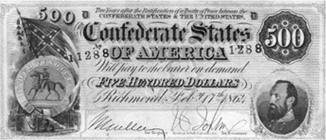
In this case, there is too much of the good, and an amount must be destroyed to make the initial price zero. Since the initial price is zero, the good is valueless at time zero, and destruction of the good makes sense—at the current quantity, the good is too costly to store for future profits. Enough is destroyed to ensure indifference between holding the good as a collectible and destroying it. Consider, for example, the $500 Confederate bill shown in Figure 11.5 "$500 Confederate States bill". Many of these bills were destroyed at the end of the U.S. Civil War, when the currency became valueless and was burned as a source of heat. Now, an uncirculated version retails for $900.

The amount of the good that must be destroyed is such that the initial price is zero. As q₀ is the initial (predestruction) quantity, the amount at time zero after the destruction is the quantity q(0) satisfying

$$0=p(0)={\left(\frac{a}{q(0)}\right)}^{\raisebox{1ex}{$1$}\!\left/ \!\raisebox{-1ex}{$\epsilon $}\right.}\frac{1}{r+\delta -\frac{\delta +g}{\epsilon }}-\frac{1}{(r+\delta )}s\text{.}$$

Given this construction, we have that

$$p(0)+\frac{1}{(r+\delta )}s-{\left(\frac{a}{q(0)}\right)}^{\raisebox{1ex}{$1$}\!\left/ \!\raisebox{-1ex}{$\epsilon $}\right.}\frac{1}{r+\delta -\frac{\delta +g}{\epsilon }}=0$$

where either q(0) = q₀ and p(0) ≥ 0, or q(0) < q₀ and p(0) = 0.

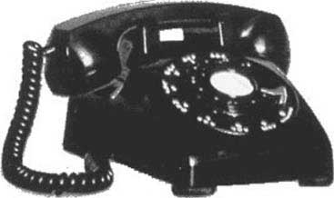
Destruction of a portion of the stock of a collectible, followed by price increases, is actually a quite common phenomenon. In particular, consider the “Model 500” telephone by Western Electric illustrated in Figure 11.6 "Western Electric Model 500 telephone". This ubiquitous classic phone was retired as the United States switched to tone dialing and push-button phones in the 1970s, and millions of phones—perhaps over 100 million—wound up in landfills. Now the phone is a collectible, and rotary phone enthusiasts work to keep them operational.

The solution for p(0) dramatically simplifies the expression for p(t):

$$p(t)=e^{(r+\delta )t}\left(p(0)+\frac{1-e^{-(r+\delta )t}}{(r+\delta )}s-{\left(\frac{a}{q(0)}\right)}^{\raisebox{1ex}{$1$}\!\left/ \!\raisebox{-1ex}{$\epsilon $}\right.}\frac{1-e^{-\left(r+\delta -\frac{\delta +g}{\epsilon }\right)t}}{r+\delta -\frac{\delta +g}{\epsilon }}\right)$$ $$=e^{(r+\delta )t}\left(\frac{-e^{-(r+\delta )t}}{(r+\delta )}s+{\left(\frac{a}{q(0)}\right)}^{\raisebox{1ex}{$1$}\!\left/ \!\raisebox{-1ex}{$\epsilon $}\right.}\frac{e^{-\left(r+\delta -\frac{\delta +g}{\epsilon }\right)t}}{r+\delta -\frac{\delta +g}{\epsilon }}\right)$$ $$={\left(\frac{a}{q(0)}\right)}^{\raisebox{1ex}{$1$}\!\left/ \!\raisebox{-1ex}{$\epsilon $}\right.}\frac{e^{\frac{\delta +g}{\epsilon }t}}{r+\delta -\frac{\delta +g}{\epsilon }}-\frac{s}{r+\delta }$$

This formula enables one to compare different collectibles. The first insight is that storage costs enter linearly into prices, so that growth rates are approximately unaffected by storage costs. The fact that gold is easy to store—while stamps and art require control of humidity and temperature in order to preserve value, and are hence more expensive to store—affects the level of prices but not the growth rate. However, depreciation and the growth of population affect the growth rate, and they do so in combination with the demand elasticity. With more elastic demand, prices grow more slowly and start at a lower level.

11.7 Summer Wheat

Typically, wheat harvested in the fall has to last until the following harvest. How should prices evolve over the season? If I know that I need wheat in January, should I buy it at harvest time and store it myself, or wait and buy it in January? We can use a theory analogous to the theory of collectibles developed in Section 11.6 "Collectibles" to determine the evolution of prices for commodities like wheat, corn, orange juice, and canola oil.

Unlike collectibles, buyers need not hold commodities for their personal use, since there is no value in admiring the wheat in your home. Let p(t) be the price at time t, and suppose that the year has length T. Generally there is a substantial amount of uncertainty regarding the size of wheat harvests, and most countries maintain an excess inventory as a precaution. However, if the harvest were not uncertain, there would be no need for a precautionary holding. Instead, we would consume the entire harvest over the course of a year, at which point the new harvest would come in. It is this such model that is investigated in this section.

Let δ represent the depreciation rate (which, for wheat, includes the quantity eaten by rodents), and let s be the storage cost. Buying at time t and reselling at t + Δ should be a break-even proposition. If one purchases at time t, it costs p(t) to buy the good. Reselling at t + Δ, the storage cost is about sΔ. (This is not the precisely relevant cost; but rather it is the present value of the storage cost, and hence the restriction to small values of Δ.) The good depreciates to only have $e^{-\delta \Delta }$ left to sell, and discounting reduces the value of that amount by the factor $e^{-r\Delta }\text{.}$ For this to be a break-even proposition, for small Δ,

$$0=e^{-r\Delta }{e}^{-\delta \Delta }p(t+\Delta )-s\Delta -p(t)$$

or

$$\frac{p(t+\Delta )-p(t)}{\Delta }=\frac{1-e^{-(r+\delta )\Delta }}{\Delta }p(t+\Delta )+s$$

taking the limit as Δ → 0, $p^{\prime }(t)=(r+\delta )p(t)+s\text{.}$

This arbitrage condition ensures that it is a break-even proposition to invest in the good; the profits from the price appreciation are exactly balanced by depreciation, interest, and storage costs. We can solve the differential equation to obtain

$$p(t)=e^{(r+\delta )t}\left(p(0)+\frac{1-e^{-(r+\delta )t}}{r+\delta }s\right)=e^{(r+\delta )t}p(0)+\frac{e^{(r+\delta )t}-1}{r+\delta }s.$$

The unknown is p(0). The constraint on p(0), however, is like the resource extraction problem—p(0) is determined by the need to use up the harvest over the course of the year.

Suppose demand has constant elasticity ε. Then the quantity used comes in the form $x(t)=ap{(t)}^{-\epsilon }\text{.}$ Let z(t) represent the stock at time t. Then the equation for the evolution of the stock is $z^{\prime }(t)=-x(t)-\delta z(t).$ This equation is obtained by noting that the flow out of stock is composed of two elements: depreciation, δz, and consumption, x. The stock evolution equation solves for

$$z(t)=e^{-\delta t}\left(q(0)-{\displaystyle \underset{0}{\overset{t}{\int }}{e}^{\delta u}x(u)du}\right)\text{.}$$

Thus, the quantity of wheat is consumed exactly if

$${\displaystyle \underset{0}{\overset{T}{\int }}{e}^{\delta u}x(u)du}=q(0)\text{.}$$

But this equation determines the initial price through

$$q(0)={\displaystyle \underset{0}{\overset{T}{\int }}{e}^{\delta u}x(u)du}={\displaystyle \underset{0}{\overset{T}{\int }}{e}^{\delta u}ap{(u)}^{-\epsilon }du}={\displaystyle \underset{0}{\overset{T}{\int }}{e}^{\delta u}a{\left(e^{(r+\delta )u}p(0)+\frac{e^{(r+\delta )u}-1}{r+\delta }s\right)}^{-\epsilon }du}\text{.}$$

This equation doesn’t lead to a closed form for p(0) but is readily estimated, which provides a practical means of computing expected prices for commodities in temporarily fixed supply.

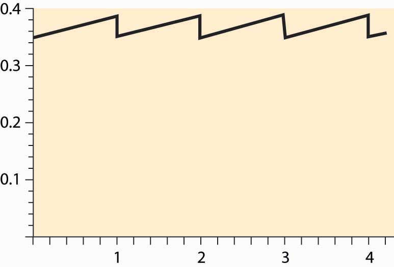
Generally, the price equation produces a “sawtooth” pattern, which is illustrated in Figure 11.7 "Prices over a cycle for seasonal commodities". The increasing portion is actually an exponential, but of such a small degree that it looks linear. When the new harvest comes in, prices drop abruptly as the inventory grows dramatically, and the same pattern is repeated.

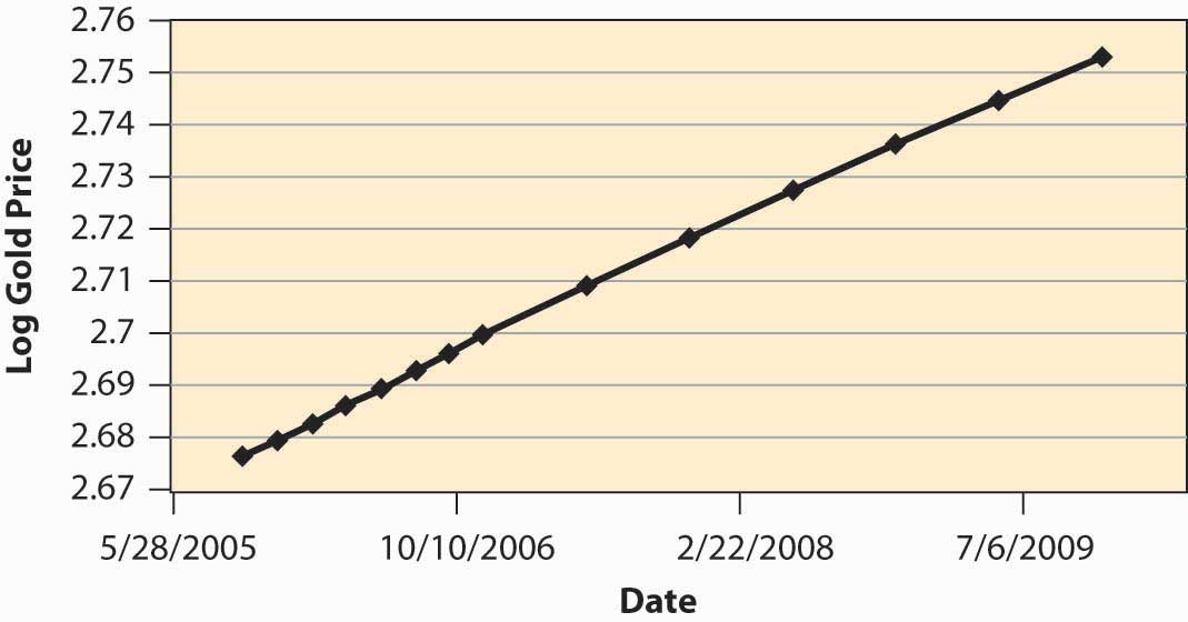
How well does the theory work? Figure 11.8 "Log of price of gold over time" shows the log of the future price of gold over time. The relevant data come from a futures market that establishes, at one moment in time, the price of gold for future delivery, and thus represents today’s estimate of the future price of gold. These data, then, represent the expected future price at a particular moment in time (the afternoon of October 11, 2005), and thus correspond to the prices in the theory, since perceived risks are fixed. (Usually, in the real world, risk plays a salient role.) We can observe that prices are approximately an exponential, because the log of prices is approximately linear. However, the estimate of r + δ is surprisingly low, at an annual level of less than 0.03, or 3% for both discounting and depreciation. Depreciation of gold is low, but this still represents a very low interest rate.