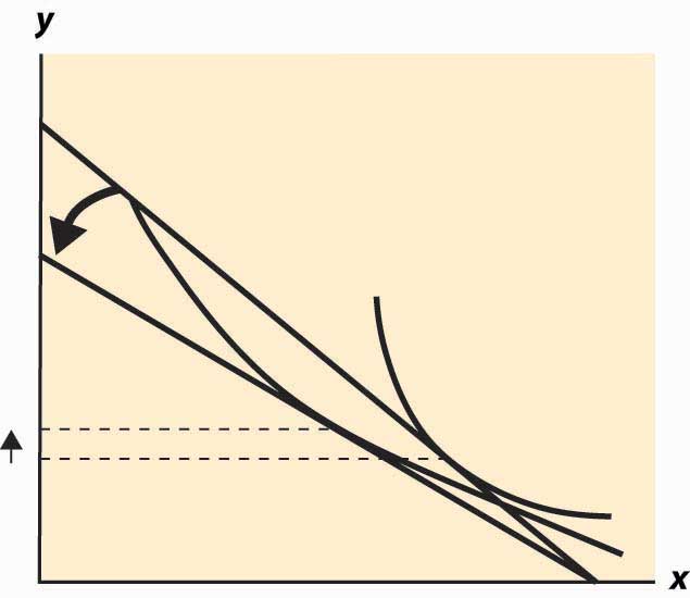
It would be a simpler world if an increase in the price of a good always entailed buying less of it. Alas, it isn’t so, as Figure 12.9 "Substitution with an increase in price" illustrates. In this figure, an increase in the price of Y causes the budget line to pivot around the intersection on the x-axis, since the amount of X that can be purchased hasn’t changed. In this case, the quantity y of Y demanded rises.
Figure 12.9 Substitution with an increase in price

At first glance, this increase in the consumption of a good in response to a price increase sounds implausible, but there are examples where it makes sense. The primary example is leisure. As wages rise, the cost of leisure (forgone wages) rises. But as people feel wealthier, they choose to work fewer hours. The other examples given, which are hotly debated in the “tempest in a teapot” kind of way, involve people subsisting on a good like potatoes but occasionally buying meat. When the price of potatoes rises, they can no longer afford meat and buy even more potatoes than before.
Thus, the logical starting point on substitution—what happens to the demand for a good when the price of that good increases—does not lead to a useful theory. As a result, economists have devised an alternative approach based on the following logic. An increase in the price of a good is really a composition of two effects: an increase in the relative price of the good and a decrease in the purchasing power of money. As a result, it is useful to examine these two effects separately. The substitution effectThe effect on consumption of a change in the relative price, with a sufficient change in income to keep the consumer on the same utility isoquant. considers the change in the relative price, with a sufficient change in income to keep the consumer on the same utility isoquant.Some authors instead change the income enough to make the old bundle affordable. This approach has the virtue of being readily computed, but the disadvantage is that the substitution effect winds up increasing the utility of the consumer. Overall the present approach is more economical for most purposes. The income effect changes only income.
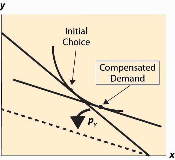
Figure 12.10 Substitution effect

To graphically illustrate the substitution effect, consider Figure 12.10 "Substitution effect". The starting point is the tangency between the isoquant and the budget line, denoted with a diamond shape and labeled “Initial Choice.” The price of Y rises, pivoting the budget line inward. The new budget line is illustrated with a heavy, dashed line. To find the substitution effect, increase income from the dashed line until the original isoquant is reached. Increases in income shift the budget line out in a fashion parallel to the original. We reach the original isoquant at a point labeled with a small circle, a point sometimes called the compensated demandDemand that exists when a change in price is accompanied by just enough additional income to keep utility the same. because we have compensated the consumer for the price increase by increasing income just enough to leave her unharmed, on the same isoquant. The substitution effect is just the difference between these points—the substitution in response to the price change, holding constant the utility of the consumer.
We can readily see that the substitution effect of a price increase in Y is to decrease the consumption of Y and increase the consumption of X.To construct a formal proof, first show that if pY rises and y rises, holding utility constant, the initial choice prior to the price increase is feasible after the price increase. Use this to conclude that, after the price increase, it is possible to have strictly more of both goods, contradicting the hypothesis that utility was held constant. The income effectThe effect on consumption of a change in income. is the change in consumption resulting from the change in income. The effect of any change in price can be decomposed into the substitution effect, which holds utility constant while changing and the income effect, which adjusts for the loss of purchasing power arising from the price increase.
Example (Cobb-Douglas): Recall that the Cobb-Douglas utility comes in the form Solving for x, y we obtain
and
Thus, consider a multiplicative increase Δ in pY—that is, multiplying pY by Δ > 1. In order to leave the utility constant, M must rise by Δ1 –α. Thus, x rises by the factor Δ1 –α and y falls by the factor Δ–α < 1. This is the substitution effect.
What is the substitution effect of a small change in the price pY for any given utility function, not necessarily Cobb-Douglas? To address this question, it is helpful to introduce some notation. We will subscript the utility to indicate partial derivative; that is,
Note that, by the definition of the substitution effect, we are holding the utility constant, so u(x, y) is being held constant. This means, locally, that Writing dx for an unknown infinitesimal change in x can be put on a formal basis. The easiest way to do so is to think of dx as representing the derivative of x with respect to a parameter, which will be pY.
In addition, we have so
Finally, we have the optimality condition which is convenient to write as Differentiating this equation, and letting we have
For a given dpY, we now have three equations in three unknowns: dx, dy, and dM. However, dM only appears in one of the three. Thus, the effect of a price change on x and y can be solved by solving two equations: and for the two unknowns, dx and dy. This is straightforward and yields
These equations imply that x rises and y falls.This is a consequence of the fact that which follows from the already stated second-order condition for a maximum of utility. We immediately see that
Thus, the change in (x, y) follows the budget line locally. (This is purely a consequence of holding utility constant.)
To complete the thought while we are embroiled in these derivatives, note that implies that
Thus, the amount of money necessary to compensate the consumer for the price increase, keeping utility constant, can be calculated from our third equation:
The amount of income necessary to ensure that the consumer makes no losses from a price increase in Y is the amount that lets him or her buy the bundle that he or she originally purchased; that is, the increase in the amount of money is precisely the amount needed to cover the increased price of y. This shows that locally there is no difference between a substitution effect that keeps utility constant (which is what we explored) and one that provides sufficient income to permit purchasing the previously purchased consumption bundle, at least when small changes in prices are contemplated.