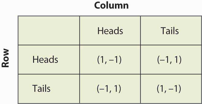
Let us consider the matching pennies game again, as illustrated in Figure 16.13 "Matching pennies again".
Figure 16.13 Matching pennies again
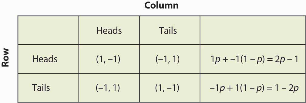
Suppose that Row believes Column plays Heads with probability p. Then if Row plays Heads, Row gets 1 with probability p and –1 with probability (1 – p), for an expected value of 2p – 1. Similarly, if Row plays Tails, Row gets –1 with probability p (when Column plays Heads), and 1 with probability (1 – p), for an expected value of 1 – 2p. This is summarized in Figure 16.14 "Mixed strategy in matching pennies".
If 2p – 1 > 1 – 2p, then Row is better off, on average, playing Heads than Tails. Similarly, if 2p – 1 < 1 – 2p, then Row is better off playing Tails than Heads. If, on the other hand, 2p – 1 = 1 – 2p, then Row gets the same payoff no matter what Row does. In this case, Row could play Heads, could play Tails, or could flip a coin and randomize Row’s play.
A mixed strategy Nash equilibriumA Nash equilibrium in which at least one player plays a randomized strategy and no player is able to increase his or her expected payoff by playing an alternate strategy. involves at least one player playing a randomized strategy and no player being able to increase his or her expected payoff by playing an alternate strategy. A Nash equilibrium in which no player randomizes is called a pure strategy Nash equilibriumA Nash equilibrium in which no player randomizes..
Figure 16.14 Mixed strategy in matching pennies
Note that randomization requires equality of expected payoffs. If a player is supposed to randomize over strategy A or strategy B, then both of these strategies must produce the same expected payoff. Otherwise, the player would prefer one of them and wouldn’t play the other.
Computing a mixed strategy has one element that often appears confusing. Suppose that Row is going to randomize. Then Row’s payoffs must be equal for all strategies that Row plays with positive probability. But that equality in Row’s payoffs doesn’t determine the probabilities with which Row plays the various rows. Instead, that equality in Row’s payoffs will determine the probabilities with which Column plays the various columns. The reason is that it is Column’s probabilities that determine the expected payoffs for Row; if Row is going to randomize, then Column’s probabilities must be such that Row is willing to randomize.
Thus, for example, we computed the payoff to Row of playing Heads, which was 2p – 1, where p was the probability that Column played Heads. Similarly, the payoff to Row of playing Tails was 1 – 2p. Row is willing to randomize if these are equal, which solves for p = ½.
Now let’s try a somewhat more challenging example and revisit the battle of the sexes. Figure 16.15 "Mixed strategy in battle of the sexes" illustrates the payoffs once again.
Figure 16.15 Mixed strategy in battle of the sexes
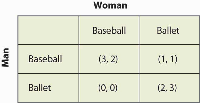
This game has two pure strategy Nash equilibria: (Baseball, Baseball) and (Ballet, Ballet). Is there a mixed strategy? To compute a mixed strategy, let the Woman go to the Baseball game with probability p, and the Man go to the Baseball game with probability q. Figure 16.16 "Full computation of the mixed strategy" contains the computation of the mixed strategy payoffs for each player.
Figure 16.16 Full computation of the mixed strategy

For example, if the Man (row player) goes to the Baseball game, he gets 3 when the Woman goes to the Baseball game (probability p), and otherwise gets 1, for an expected payoff of 3p + 1(1 – p) = 1 + 2p. The other calculations are similar, but you should definitely run through the logic and verify each calculation.
A mixed strategy in the battle of the sexes game requires both parties to randomize (since a pure strategy by either party prevents randomization by the other). The Man’s indifference between going to the Baseball game and to the Ballet requires 1 + 2p = 2 – 2p, which yields p = ¼. That is, the Man will be willing to randomize which event he attends if the Woman is going to the Ballet ¾ of the time, and otherwise to the Baseball game. This makes the Man indifferent between the two events because he prefers to be with the Woman, but he also likes to be at the Baseball game. To make up for the advantage that the game holds for him, the Woman has to be at the Ballet more often.
Similarly, in order for the Woman to randomize, the Woman must get equal payoffs from going to the Baseball game and going to the Ballet, which requires 2q = 3 – 2q, or q = ¾. Thus, the probability that the Man goes to the Baseball game is ¾, and he goes to the Ballet ¼ of the time. These are independent probabilities, so to get the probability that both go to the Baseball game, we multiply the probabilities, which yields 3/16. Figure 16.17 "Mixed strategy probabilities" fills in the probabilities for all four possible outcomes.
Figure 16.17 Mixed strategy probabilities
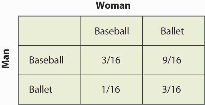
Note that more than half of the time (Baseball, Ballet) is the outcome of the mixed strategy and the two people are not together. This lack of coordination is generally a feature of mixed strategy equilibria. The expected payoffs for both players are readily computed as well. The Man’s payoff is 1 + 2p = 2 – 2p, and since p = ¼, the Man obtains 1½. A similar calculation shows that the Woman’s payoff is the same. Thus, both do worse than coordinating on their less preferred outcome. But this mixed strategy Nash equilibrium, undesirable as it may seem, is a Nash equilibrium in the sense that neither party can improve his or her own payoff, given the behavior of the other party.
In the battle of the sexes, the mixed strategy Nash equilibrium may seem unlikely; and we might expect the couple to coordinate more effectively. Indeed, a simple call on the telephone should rule out the mixed strategy. So let’s consider another game related to the battle of the sexes, where a failure of coordination makes more sense. This is the game of “chicken.” In this game, two players drive toward one another, trying to convince the other to yield and ultimately swerve into a ditch. If both swerve into the ditch, we’ll call the outcome a draw and both get zero. If one swerves and the other doesn’t, the driver who swerves loses and the other driver wins, and we’ll give the winner one point.Note that adding a constant to a player’s payoffs, or multiplying that player’s payoffs by a positive constant, doesn’t affect the Nash equilibria—pure or mixed. Therefore, we can always let one outcome for each player be zero, and another outcome be one. The only remaining question is what happens when neither yield, in which case a crash results. In this version, the payoff has been set at four times the loss of swerving, as shown in Figure 16.18 "Chicken", but you can change the game and see what happens.
Figure 16.18 Chicken
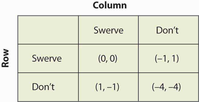
This game has two pure strategy equilibria: (Swerve, Don’t) and (Don’t, Swerve). In addition, it has a mixed strategy. Suppose that Column swerves with probability p. Then Row gets 0p + –1(1 – p) from swerving, 1p + (–4)(1 – p) from not swerving, and Row will randomize if these are equal, which requires p = ¾. That is, the probability that Column swerves in a mixed strategy equilibrium is ¾. You can verify that the row player has the same probability by setting the probability that Row swerves equal to q and computing Column’s expected payoffs. Thus, the probability of a collision is 1/16 in the mixed strategy equilibrium.
The mixed strategy equilibrium is more likely, in some sense, in this game: If the players already knew who was going to yield, they wouldn’t actually need to play the game. The whole point of the game is to find out who will yield, which means that it isn’t known in advance. This means that the mixed strategy equilibrium is, in some sense, the more reasonable equilibrium.
Figure 16.19 Rock, paper, scissors
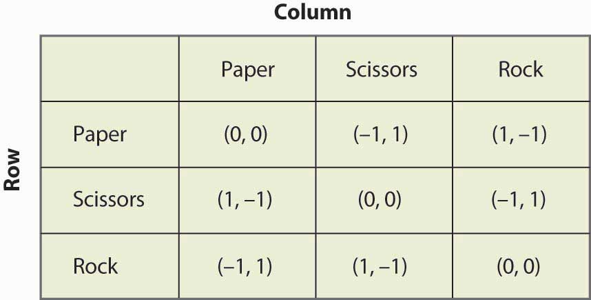
“Rock, paper, scissors” is a child’s game in which two children use their hands to simultaneously choose paper (hand held flat), scissors (hand with two fingers protruding to look like scissors), or rock (hand in a fist). The nature of the payoffs is that paper beats rock, rock beats scissors, and scissors beats paper. This game has the structure that is illustrated in Figure 16.19 "Rock, paper, scissors".
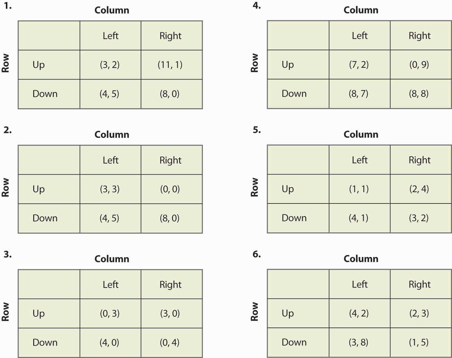
Find all equilibria of the following games:
Figure 16.20
