The Empirical Rule and Chebyshev’s Theorem

2.5 The Empirical Rule and Chebyshev’s Theorem

Learning Objectives

To learn what the value of the standard deviation of a data set implies about how the data scatter away from the mean as described by the Empirical Rule and Chebyshev’s Theorem.
To use the Empirical Rule and Chebyshev’s Theorem to draw conclusions about a data set.

You probably have a good intuitive grasp of what the average of a data set says about that data set. In this section we begin to learn what the standard deviation has to tell us about the nature of the data set.

The Empirical Rule

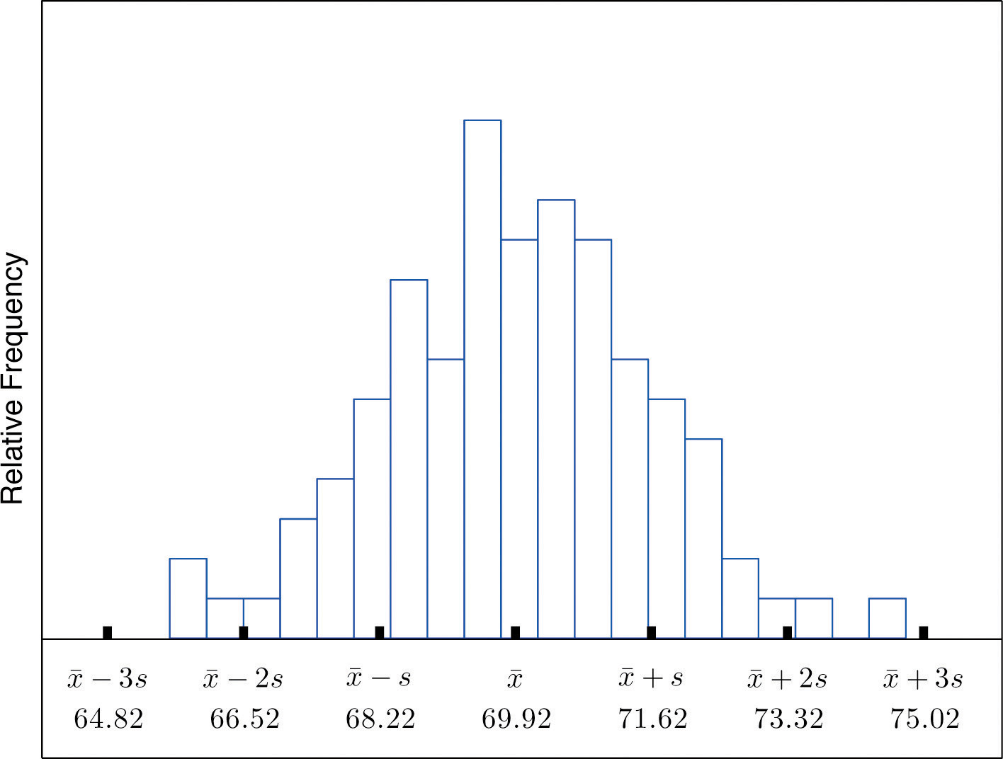
We start by examining a specific set of data. Table 2.2 "Heights of Men" shows the heights in inches of 100 randomly selected adult men. A relative frequency histogram for the data is shown in Figure 2.15 "Heights of Adult Men". The mean and standard deviation of the data are, rounded to two decimal places, $\bar{x} = 69.92$ and s = 1.70. If we go through the data and count the number of observations that are within one standard deviation of the mean, that is, that are between $69.92 - 1.70 = 68.22$ and $69.92 + 1.70 = 71.62$ inches, there are 69 of them. If we count the number of observations that are within two standard deviations of the mean, that is, that are between $69.92 - 2 (1.70) = 66.52$ and $69.92 + 2 (1.70) = 73.32$ inches, there are 95 of them. All of the measurements are within three standard deviations of the mean, that is, between $69.92 - 3 (1.70) = 64.822$ and $69.92 + 3 (1.70) = 75.02$ inches. These tallies are not coincidences, but are in agreement with the following result that has been found to be widely applicable.

Table 2.2 Heights of Men

68.7	72.3	71.3	72.5	70.6	68.2	70.1	68.4	68.6	70.6
73.7	70.5	71.0	70.9	69.3	69.4	69.7	69.1	71.5	68.6
70.9	70.0	70.4	68.9	69.4	69.4	69.2	70.7	70.5	69.9
69.8	69.8	68.6	69.5	71.6	66.2	72.4	70.7	67.7	69.1
68.8	69.3	68.9	74.8	68.0	71.2	68.3	70.2	71.9	70.4
71.9	72.2	70.0	68.7	67.9	71.1	69.0	70.8	67.3	71.8
70.3	68.8	67.2	73.0	70.4	67.8	70.0	69.5	70.1	72.0
72.2	67.6	67.0	70.3	71.2	65.6	68.1	70.8	71.4	70.2
70.1	67.5	71.3	71.5	71.0	69.1	69.5	71.1	66.8	71.8
69.6	72.7	72.8	69.6	65.9	68.0	69.7	68.7	69.8	69.7

Figure 2.15 Heights of Adult Men

The Empirical Rule

If a data set has an approximately bell-shaped relative frequency histogram, then (see Figure 2.16 "The Empirical Rule")

approximately 68% of the data lie within one standard deviation of the mean, that is, in the interval with endpoints $\bar{x} \pm s$ for samples and with endpoints $μ \pm σ$ for populations;
approximately 95% of the data lie within two standard deviations of the mean, that is, in the interval with endpoints $\bar{x} \pm 2 s$ for samples and with endpoints $μ \pm 2 σ$ for populations; and
approximately 99.7% of the data lies within three standard deviations of the mean, that is, in the interval with endpoints $\bar{x} \pm 3 s$ for samples and with endpoints $μ \pm 3 σ$ for populations.

Figure 2.16 The Empirical Rule

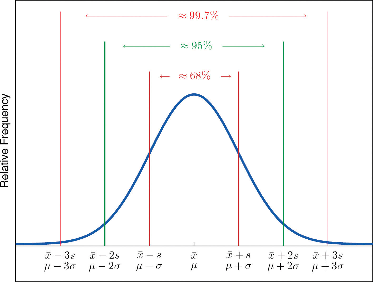
Two key points in regard to the Empirical Rule are that the data distribution must be approximately bell-shaped and that the percentages are only approximately true. The Empirical Rule does not apply to data sets with severely asymmetric distributions, and the actual percentage of observations in any of the intervals specified by the rule could be either greater or less than those given in the rule. We see this with the example of the heights of the men: the Empirical Rule suggested 68 observations between 68.22 and 71.62 inches but we counted 69.

Example 19

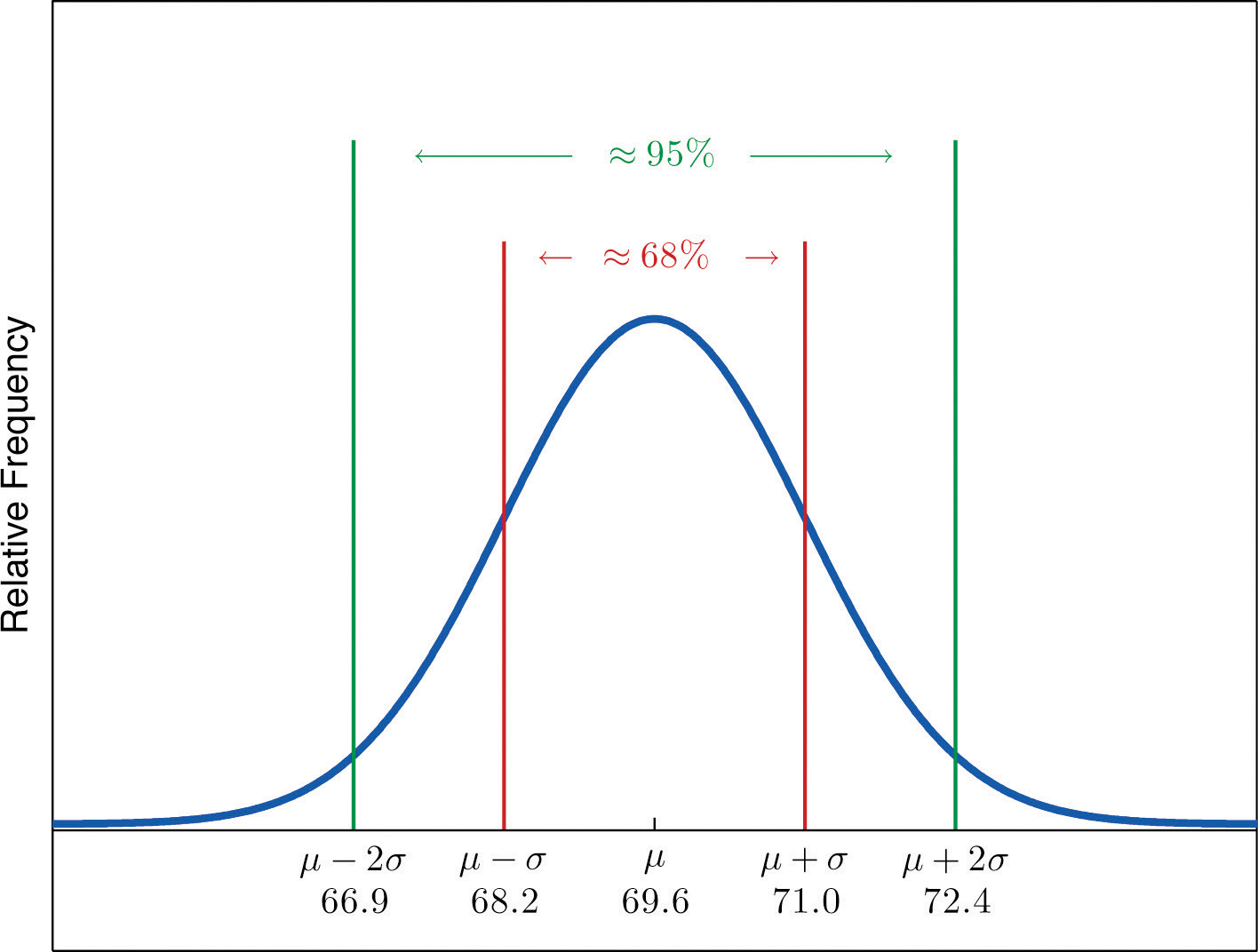
Heights of 18-year-old males have a bell-shaped distribution with mean 69.6 inches and standard deviation 1.4 inches.

About what proportion of all such men are between 68.2 and 71 inches tall?
What interval centered on the mean should contain about 95% of all such men?

Solution:

A sketch of the distribution of heights is given in Figure 2.17 "Distribution of Heights".

Since the interval from 68.2 to 71.0 has endpoints $\bar{x} - s$ and $\bar{x} + s$ , by the Empirical Rule about 68% of all 18-year-old males should have heights in this range.
By the Empirical Rule the shortest such interval has endpoints $\bar{x} − 2 s$ and $\bar{x} + 2 s .$ Since
$\bar{x} − 2 s = 69.6 - 2 (1.4) = 66.8 and \bar{x} + 2 s = 69.6 + 2 (1.4) = 72.4$
the interval in question is the interval from 66.8 inches to 72.4 inches.

Figure 2.17 Distribution of Heights

Example 20

Scores on IQ tests have a bell-shaped distribution with mean μ = 100 and standard deviation σ = 10. Discuss what the Empirical Rule implies concerning individuals with IQ scores of 110, 120, and 130.

Solution:

A sketch of the IQ distribution is given in Figure 2.18 "Distribution of IQ Scores". The Empirical Rule states that

approximately 68% of the IQ scores in the population lie between 90 and 110,
approximately 95% of the IQ scores in the population lie between 80 and 120, and
approximately 99.7% of the IQ scores in the population lie between 70 and 130.

Figure 2.18 Distribution of IQ Scores

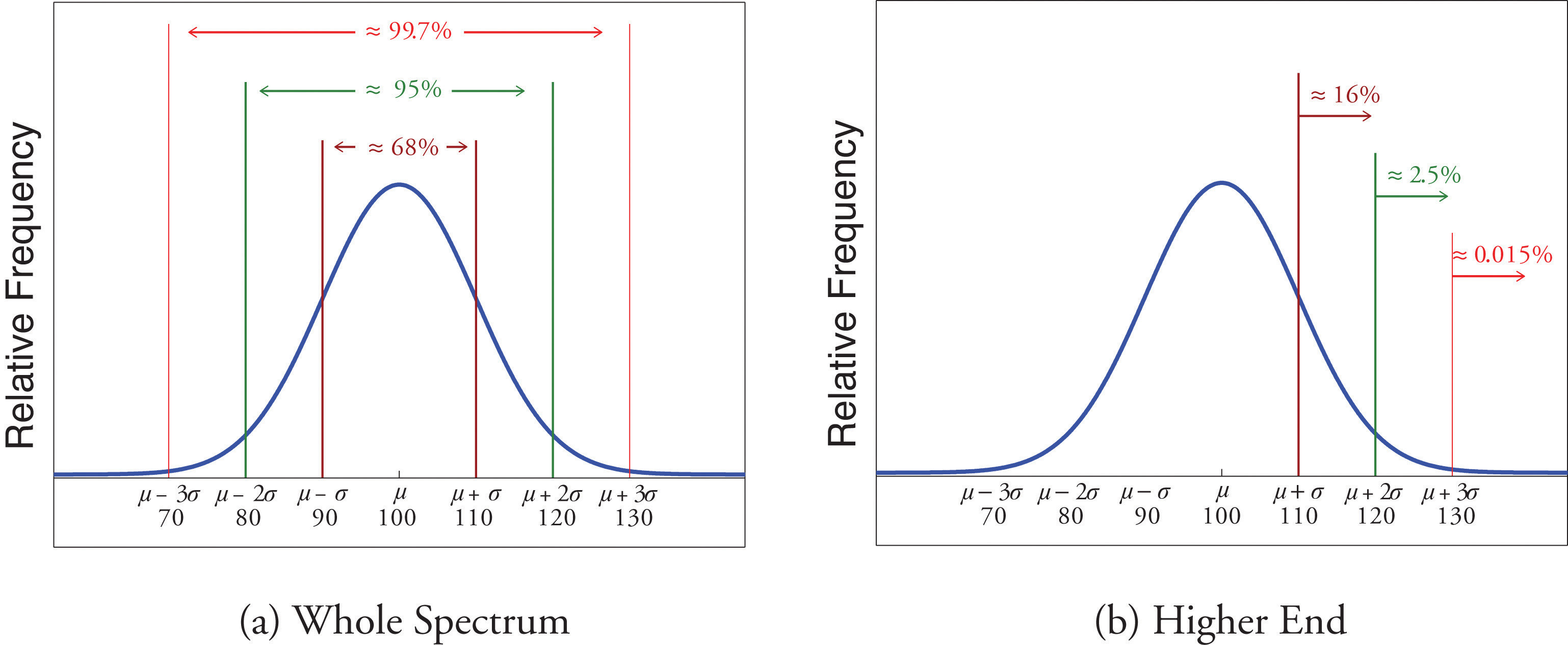
Since 68% of the IQ scores lie within the interval from 90 to 110, it must be the case that 32% lie outside that interval. By symmetry approximately half of that 32%, or 16% of all IQ scores, will lie above 110. If 16% lie above 110, then 84% lie below. We conclude that the IQ score 110 is the 84th percentile.

The same analysis applies to the score 120. Since approximately 95% of all IQ scores lie within the interval form 80 to 120, only 5% lie outside it, and half of them, or 2.5% of all scores, are above 120. The IQ score 120 is thus higher than 97.5% of all IQ scores, and is quite a high score.

By a similar argument, only 15/100 of 1% of all adults, or about one or two in every thousand, would have an IQ score above 130. This fact makes the score 130 extremely high.

Chebyshev’s Theorem

The Empirical Rule does not apply to all data sets, only to those that are bell-shaped, and even then is stated in terms of approximations. A result that applies to every data set is known as Chebyshev’s Theorem.

Chebyshev’s Theorem

For any numerical data set,

at least 3/4 of the data lie within two standard deviations of the mean, that is, in the interval with endpoints $\bar{x} \pm 2 s$ for samples and with endpoints $μ \pm 2 σ$ for populations;
at least 8/9 of the data lie within three standard deviations of the mean, that is, in the interval with endpoints $\bar{x} \pm 3 s$ for samples and with endpoints $μ \pm 3 σ$ for populations;
at least $1 - 1 ∕ k^{2}$ of the data lie within k standard deviations of the mean, that is, in the interval with endpoints $\bar{x} \pm k s$ for samples and with endpoints $μ \pm k σ$ for populations, where k is any positive whole number that is greater than 1.

Figure 2.19 "Chebyshev’s Theorem" gives a visual illustration of Chebyshev’s Theorem.

Figure 2.19 Chebyshev’s Theorem

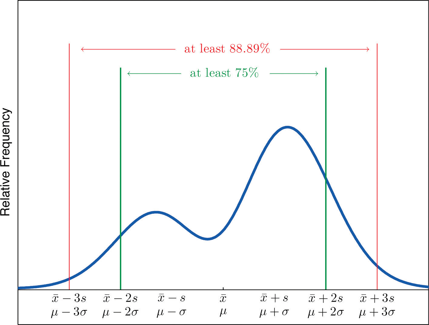
It is important to pay careful attention to the words “at least” at the beginning of each of the three parts. The theorem gives the minimum proportion of the data which must lie within a given number of standard deviations of the mean; the true proportions found within the indicated regions could be greater than what the theorem guarantees.

Example 21

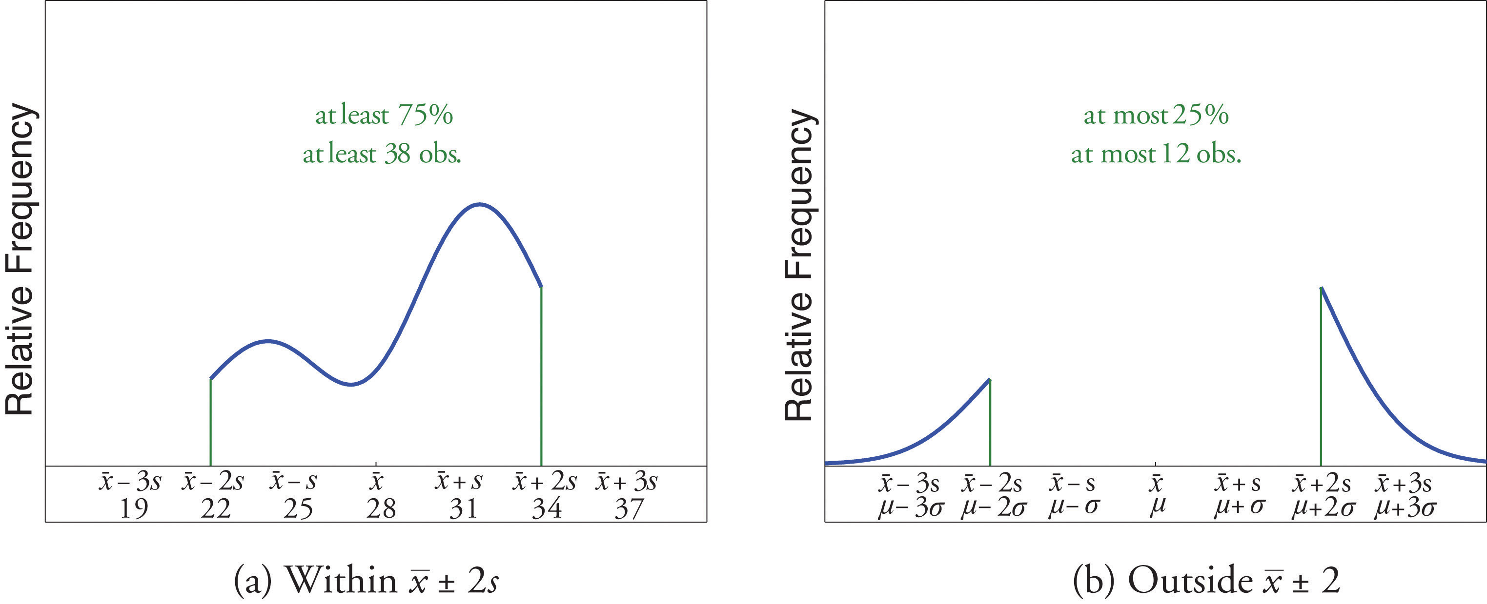
A sample of size n = 50 has mean $\bar{x} = 28$ and standard deviation s = 3. Without knowing anything else about the sample, what can be said about the number of observations that lie in the interval (22,34)? What can be said about the number of observations that lie outside that interval?

Solution:

The interval (22,34) is the one that is formed by adding and subtracting two standard deviations from the mean. By Chebyshev’s Theorem, at least 3/4 of the data are within this interval. Since 3/4 of 50 is 37.5, this means that at least 37.5 observations are in the interval. But one cannot take a fractional observation, so we conclude that at least 38 observations must lie inside the interval (22,34).

If at least 3/4 of the observations are in the interval, then at most 1/4 of them are outside it. Since 1/4 of 50 is 12.5, at most 12.5 observations are outside the interval. Since again a fraction of an observation is impossible, x (22,34).

Example 22

The number of vehicles passing through a busy intersection between 8:00 a.m. and 10:00 a.m. was observed and recorded on every weekday morning of the last year. The data set contains n = 251 numbers. The sample mean is $\bar{x} = 725$ and the sample standard deviation is s = 25. Identify which of the following statements must be true.

On approximately 95% of the weekday mornings last year the number of vehicles passing through the intersection from 8:00 a.m. to 10:00 a.m. was between 675 and 775.
On at least 75% of the weekday mornings last year the number of vehicles passing through the intersection from 8:00 a.m. to 10:00 a.m. was between 675 and 775.
On at least 189 weekday mornings last year the number of vehicles passing through the intersection from 8:00 a.m. to 10:00 a.m. was between 675 and 775.
On at most 25% of the weekday mornings last year the number of vehicles passing through the intersection from 8:00 a.m. to 10:00 a.m. was either less than 675 or greater than 775.
On at most 12.5% of the weekday mornings last year the number of vehicles passing through the intersection from 8:00 a.m. to 10:00 a.m. was less than 675.
On at most 25% of the weekday mornings last year the number of vehicles passing through the intersection from 8:00 a.m. to 10:00 a.m. was less than 675.

Solution:

Since it is not stated that the relative frequency histogram of the data is bell-shaped, the Empirical Rule does not apply. Statement (1) is based on the Empirical Rule and therefore it might not be correct.
Statement (2) is a direct application of part (1) of Chebyshev’s Theorem because $(\bar{x} − 2 s, \bar{x} + 2 s) = (675,775) .$ It must be correct.
Statement (3) says the same thing as statement (2) because 75% of 251 is 188.25, so the minimum whole number of observations in this interval is 189. Thus statement (3) is definitely correct.
Statement (4) says the same thing as statement (2) but in different words, and therefore is definitely correct.
Statement (4), which is definitely correct, states that at most 25% of the time either fewer than 675 or more than 775 vehicles passed through the intersection. Statement (5) says that half of that 25% corresponds to days of light traffic. This would be correct if the relative frequency histogram of the data were known to be symmetric. But this is not stated; perhaps all of the observations outside the interval (675,775) are less than 75. Thus statement (5) might not be correct.
Statement (4) is definitely correct and statement (4) implies statement (6): even if every measurement that is outside the interval (675,775) is less than 675 (which is conceivable, since symmetry is not known to hold), even so at most 25% of all observations are less than 675. Thus statement (6) must definitely be correct.

Key Takeaways

The Empirical Rule is an approximation that applies only to data sets with a bell-shaped relative frequency histogram. It estimates the proportion of the measurements that lie within one, two, and three standard deviations of the mean.
Chebyshev’s Theorem is a fact that applies to all possible data sets. It describes the minimum proportion of the measurements that lie must within one, two, or more standard deviations of the mean.

Exercises

Basic

State the Empirical Rule.
Describe the conditions under which the Empirical Rule may be applied.
State Chebyshev’s Theorem.
Describe the conditions under which Chebyshev’s Theorem may be applied.
A sample data set with a bell-shaped distribution has mean $\bar{x} = 6$ and standard deviation s = 2. Find the approximate proportion of observations in the data set that lie:
1. between 4 and 8;
2. between 2 and 10;
3. between 0 and 12.
A population data set with a bell-shaped distribution has mean μ = 6 and standard deviation σ = 2. Find the approximate proportion of observations in the data set that lie:
1. between 4 and 8;
2. between 2 and 10;
3. between 0 and 12.
A population data set with a bell-shaped distribution has mean μ = 2 and standard deviation σ = 1.1. Find the approximate proportion of observations in the data set that lie:
1. above 2;
2. above 3.1;
3. between 2 and 3.1.
A sample data set with a bell-shaped distribution has mean $\bar{x} = 2$ and standard deviation s = 1.1. Find the approximate proportion of observations in the data set that lie:
1. below −0.2;
2. below 3.1;
3. between −1.3 and 0.9.
A population data set with a bell-shaped distribution and size N = 500 has mean μ = 2 and standard deviation σ = 1.1. Find the approximate number of observations in the data set that lie:
1. above 2;
2. above 3.1;
3. between 2 and 3.1.
A sample data set with a bell-shaped distribution and size n = 128 has mean $\bar{x} = 2$ and standard deviation s = 1.1. Find the approximate number of observations in the data set that lie:
1. below −0.2;
2. below 3.1;
3. between −1.3 and 0.9.
A sample data set has mean $\bar{x} = 6$ and standard deviation s = 2. Find the minimum proportion of observations in the data set that must lie:
1. between 2 and 10;
2. between 0 and 12;
3. between 4 and 8.
A population data set has mean μ = 2 and standard deviation σ = 1.1. Find the minimum proportion of observations in the data set that must lie:
1. between −0.2 and 4.2;
2. between −1.3 and 5.3.
A population data set of size N = 500 has mean μ = 5.2 and standard deviation σ = 1.1. Find the minimum number of observations in the data set that must lie:
1. between 3 and 7.4;
2. between 1.9 and 8.5.
A sample data set of size n = 128 has mean $\bar{x} = 2$ and standard deviation s = 2. Find the minimum number of observations in the data set that must lie:
1. between −2 and 6 (including −2 and 6);
2. between −4 and 8 (including −4 and 8).
A sample data set of size n = 30 has mean $\bar{x} = 6$ and standard deviation s = 2.
1. What is the maximum proportion of observations in the data set that can lie outside the interval (2,10)?
2. What can be said about the proportion of observations in the data set that are below 2?
3. What can be said about the proportion of observations in the data set that are above 10?
4. What can be said about the number of observations in the data set that are above 10?
A population data set has mean μ = 2 and standard deviation σ = 1.1.
1. What is the maximum proportion of observations in the data set that can lie outside the interval $(− 1 . 3,5 . 3)$ ?
2. What can be said about the proportion of observations in the data set that are below −1.3?
3. What can be said about the proportion of observations in the data set that are above 5.3?

Applications

Scores on a final exam taken by 1,200 students have a bell-shaped distribution with mean 72 and standard deviation 9.
1. What is the median score on the exam?
2. About how many students scored between 63 and 81?
3. About how many students scored between 72 and 90?
4. About how many students scored below 54?
Lengths of fish caught by a commercial fishing boat have a bell-shaped distribution with mean 23 inches and standard deviation 1.5 inches.
1. About what proportion of all fish caught are between 20 inches and 26 inches long?
2. About what proportion of all fish caught are between 20 inches and 23 inches long?
3. About how long is the longest fish caught (only a small fraction of a percent are longer)?
Hockey pucks used in professional hockey games must weigh between 5.5 and 6 ounces. If the weight of pucks manufactured by a particular process is bell-shaped, has mean 5.75 ounces and standard deviation 0.125 ounce, what proportion of the pucks will be usable in professional games?
Hockey pucks used in professional hockey games must weigh between 5.5 and 6 ounces. If the weight of pucks manufactured by a particular process is bell-shaped and has mean 5.75 ounces, how large can the standard deviation be if 99.7% of the pucks are to be usable in professional games?
Speeds of vehicles on a section of highway have a bell-shaped distribution with mean 60 mph and standard deviation 2.5 mph.
1. If the speed limit is 55 mph, about what proportion of vehicles are speeding?
2. What is the median speed for vehicles on this highway?
3. What is the percentile rank of the speed 65 mph?
4. What speed corresponds to the 16th percentile?
Suppose that, as in the previous exercise, speeds of vehicles on a section of highway have mean 60 mph and standard deviation 2.5 mph, but now the distribution of speeds is unknown.
1. If the speed limit is 55 mph, at least what proportion of vehicles must speeding?
2. What can be said about the proportion of vehicles going 65 mph or faster?
An instructor announces to the class that the scores on a recent exam had a bell-shaped distribution with mean 75 and standard deviation 5.
1. What is the median score?
2. Approximately what proportion of students in the class scored between 70 and 80?
3. Approximately what proportion of students in the class scored above 85?
4. What is the percentile rank of the score 85?
The GPAs of all currently registered students at a large university have a bell-shaped distribution with mean 2.7 and standard deviation 0.6. Students with a GPA below 1.5 are placed on academic probation. Approximately what percentage of currently registered students at the university are on academic probation?
Thirty-six students took an exam on which the average was 80 and the standard deviation was 6. A rumor says that five students had scores 61 or below. Can the rumor be true? Why or why not?

Additional Exercises

For the sample data
$\begin{matrix} x & 26 & 27 & 28 & 29 & 30 & 31 & 32 \\ f & 3 & 4 & 16 & 12 & 6 & 2 & 1 \end{matrix}$
$Σ x = 1,256$ and $Σ x^{2} = 35,926 .$
1. Compute the mean and the standard deviation.
2. About how many of the measurements does the Empirical Rule predict will be in the interval $(\bar{x} - s, \bar{x} + s)$ , the interval $(\bar{x} − 2 s, \bar{x} + 2 s)$ , and the interval $(\bar{x} − 3 s, \bar{x} + 3 s)$ ?
3. Compute the number of measurements that are actually in each of the intervals listed in part (a), and compare to the predicted numbers.
A sample of size n = 80 has mean 139 and standard deviation 13, but nothing else is known about it.
1. What can be said about the number of observations that lie in the interval (126,152)?
2. What can be said about the number of observations that lie in the interval (113,165)?
3. What can be said about the number of observations that exceed 165?
4. What can be said about the number of observations that either exceed 165 or are less than 113?
For the sample data
$\begin{matrix} x & 1 & 2 & 3 & 4 & 5 \\ f & 84 & 29 & 3 & 3 & 1 \end{matrix}$
$Σ x = 168$ and $Σ x^{2} = 300 .$
1. Compute the sample mean and the sample standard deviation.
2. Considering the shape of the data set, do you expect the Empirical Rule to apply? Count the number of measurements within one standard deviation of the mean and compare it to the number predicted by the Empirical Rule.
3. What does Chebyshev’s Rule say about the number of measurements within one standard deviation of the mean?
4. Count the number of measurements within two standard deviations of the mean and compare it to the minimum number guaranteed by Chebyshev’s Theorem to lie in that interval.
For the sample data set
$\begin{matrix} x & 47 & 48 & 49 & 50 & 51 \\ f & 1 & 3 & 18 & 2 & 1 \end{matrix}$
$Σ x = 1224$ and $Σ x^{2} = 59,940 .$
1. Compute the sample mean and the sample standard deviation.
2. Considering the shape of the data set, do you expect the Empirical Rule to apply? Count the number of measurements within one standard deviation of the mean and compare it to the number predicted by the Empirical Rule.
3. What does Chebyshev’s Rule say about the number of measurements within one standard deviation of the mean?
4. Count the number of measurements within two standard deviations of the mean and compare it to the minimum number guaranteed by Chebyshev’s Theorem to lie in that interval.

Answers

See the displayed statement in the text.
See the displayed statement in the text.
1. 0.68.
2. 0.95.
3. 0.997.
1. 0.5.
2. 0.16.
3. 0.34.
1. 250.
2. 80.
3. 170.
1. 3/4.
2. 8/9.
3. 0.
1. 375.
2. 445.
1. At most 0.25.
2. At most 0.25.
3. At most 0.25.
4. At most 7.

1. 72.
2. 816.
3. 570.
4. 30.
0.95.
1. 0.975.
2. 60.
3. 97.5.
4. 57.5.
1. 75.
2. 0.68.
3. 0.025.
4. 0.975.
By Chebyshev’s Theorem at most 1∕9 of the scores can be below 62, so the rumor is impossible.

1. Nothing.
2. It is at least 60.
3. It is at most 20.
4. It is at most 20.
1. $\bar{x} = 48.96$ , s = 0.7348.
2. Roughly bell-shaped, the Empirical Rule should apply. True count: 18, predicted: 17.
3. Nothing.
4. True count: 23, guaranteed: at least 18.75, hence at least 19.