Comparison of Two Population Means: Small, Independent Samples

9.2 Comparison of Two Population Means: Small, Independent Samples

Learning Objectives

To learn how to construct a confidence interval for the difference in the means of two distinct populations using small, independent samples.
To learn how to perform a test of hypotheses concerning the difference between the means of two distinct populations using small, independent samples.

When one or the other of the sample sizes is small, as is often the case in practice, the Central Limit Theorem does not apply. We must then impose conditions on the population to give statistical validity to the test procedure. We will assume that both populations from which the samples are taken have a normal probability distribution and that their standard deviations are equal.

Confidence Intervals

When the two populations are normally distributed and have equal standard deviations, the following formula for a confidence interval for $μ_{1} - μ_{2}$ is valid.

$100 (1 - α) %$ Confidence Interval for the Difference Between Two Population Means: Small, Independent Samples

\begin{matrix} ({\bar{x}}_{1} - {\bar{x}}_{2}) \pm t_{α ∕ 2} \sqrt{s_{p}^{2} (\frac{1}{n_{1}} + \frac{1}{n_{2}})} & where & s_{p}^{2} = \frac{(n_{1} − 1) s_{1}^{2} + (n_{2} − 1) s_{2}^{2}}{n_{1} + n_{2} − 2} \end{matrix}

The number of degrees of freedom is $d f = n_{1} + n_{2} − 2 .$

The samples must be independent, the populations must be normal, and the population standard deviations must be equal. “Small” samples means that either $n_{1} < 30$ or $n_{2} < 30 .$

The quantity $s_{p}^{2}$ is called the pooled sample variance. It is a weighted average of the two estimates $s_{1}^{2}$ and $s_{2}^{2}$ of the common variance $σ_{1}^{2} = σ_{2}^{2}$ of the two populations.

Example 4

A software company markets a new computer game with two experimental packaging designs. Design 1 is sent to 11 stores; their average sales the first month is 52 units with sample standard deviation 12 units. Design 2 is sent to 6 stores; their average sales the first month is 46 units with sample standard deviation 10 units. Construct a point estimate and a 95% confidence interval for the difference in average monthly sales between the two package designs.

Solution:

The point estimate of $μ_{1} - μ_{2}$ is

{\bar{x}}_{1} - {\bar{x}}_{2} = 52 - 46 = 6

In words, we estimate that the average monthly sales for Design 1 is 6 units more per month than the average monthly sales for Design 2.

To apply the formula for the confidence interval, we must find $t_{α ∕ 2} .$ The 95% confidence level means that α = 1 − 0.95 = 0.05 so that $t_{α ∕ 2} = t_{0.025} .$ From Figure 12.3 "Critical Values of ", in the row with the heading df = 11 + 6 − 2 = 15 we read that $t_{0.025} = 2.131 .$ From the formula for the pooled sample variance we compute

s_{p}^{2} = \frac{(n_{1} − 1) s_{1}^{2} + (n_{2} − 1) s_{2}^{2}}{n_{1} + n_{2} − 2} = \frac{(10) {(12)}^{2} + (5) {(10)}^{2}}{15} = 129 . \bar{3}

Thus

({\bar{x}}_{1} - {\bar{x}}_{2}) \pm t_{α ∕ 2} \sqrt{s_{p}^{2} (\frac{1}{n_{1}} + \frac{1}{n_{2}})} = 6 \pm (2.131) \sqrt{129. \bar{3} (\frac{1}{11} + \frac{1}{6})} \approx 6 \pm 12.3

We are 95% confident that the difference in the population means lies in the interval $[− 6 . 3,18 . 3]$ , in the sense that in repeated sampling 95% of all intervals constructed from the sample data in this manner will contain $μ_{1} - μ_{2} .$ Because the interval contains both positive and negative values the statement in the context of the problem is that we are 95% confident that the average monthly sales for Design 1 is between 18.3 units higher and 6.3 units lower than the average monthly sales for Design 2.

Hypothesis Testing

Testing hypotheses concerning the difference of two population means using small samples is done precisely as it is done for large samples, using the following standardized test statistic. The same conditions on the populations that were required for constructing a confidence interval for the difference of the means must also be met when hypotheses are tested.

Standardized Test Statistic for Hypothesis Tests Concerning the Difference Between Two Population Means: Small, Independent Samples

\begin{matrix} T = \frac{({\bar{x}}_{1} - {\bar{x}}_{2}) - D_{0}}{\sqrt{s_{p}^{2} (\frac{1}{n_{1}} + \frac{1}{n_{2}})}} & where & s_{p}^{2} = \frac{(n_{1} − 1) s_{1}^{2} + (n_{2} − 1) s_{2}^{2}}{n_{1} + n_{2} − 2} \end{matrix}

The test statistic has Student’s t-distribution with $d f = n_{1} + n_{2} − 2$ degrees of freedom.

The samples must be independent, the populations must be normal, and the population standard deviations must be equal. “Small” samples means that either $n_{1} < 30$ or $n_{2} < 30 .$

Example 5

Refer to Note 9.11 "Example 4" concerning the mean sales per month for the same computer game but sold with two package designs. Test at the 1% level of significance whether the data provide sufficient evidence to conclude that the mean sales per month of the two designs are different. Use the critical value approach.

Solution:

Step 1. The relevant test is
$\begin{matrix} H_{0} : μ_{1} - μ_{2} & = & 0 \\ vs. H_{a} : μ_{1} - μ_{2} & \neq & 0 & @ α = 0.01 \end{matrix}$
Step 2. Since the samples are independent and at least one is less than 30 the test statistic is
$T = \frac{({\bar{x}}_{1} - {\bar{x}}_{2}) - D_{0}}{\sqrt{s_{p}^{2} (\frac{1}{n_{1}} + \frac{1}{n_{2}})}}$
which has Student’s t-distribution with $d f = 11 + 6 - 2 = 15$ degrees of freedom.
Step 3. Inserting the data and the value $D_{0} = 0$ into the formula for the test statistic gives
$T = \frac{({\bar{x}}_{1} - {\bar{x}}_{2}) - D_{0}}{\sqrt{s_{p}^{2} (\frac{1}{n_{1}} + \frac{1}{n_{2}})}} = \frac{(52 - 46) − 0}{\sqrt{129. \bar{3} (\frac{1}{11} + \frac{1}{6})}} = 1.040$
Step 4. Since the symbol in H_a is “≠” this is a two-tailed test, so there are two critical values, $\pm t_{α ∕ 2} = \pm t_{0.005} .$ From the row in Figure 12.3 "Critical Values of " with the heading $d f = 15$ we read off $t_{0.005} = 2.947 .$ The rejection region is $(− \infty, − 2.947] \cup [2.947, \infty) .$

Figure 9.4 Rejection Region and Test Statistic for Note 9.13 "Example 5"
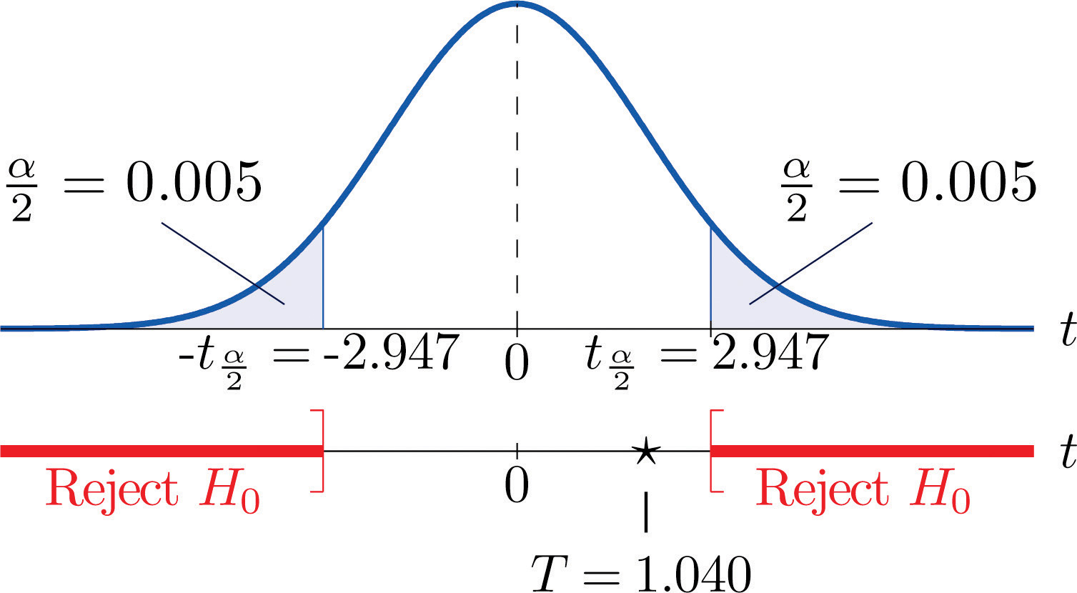
Step 5. As shown in Figure 9.4 "Rejection Region and Test Statistic for " the test statistic does not fall in the rejection region. The decision is not to reject H₀. In the context of the problem our conclusion is:

The data do not provide sufficient evidence, at the 1% level of significance, to conclude that the mean sales per month of the two designs are different.

Example 6

Perform the test of Note 9.13 "Example 5" using the p-value approach.

Solution:

The first three steps are identical to those in Note 9.13 "Example 5".

Step 4. Because the test is two-tailed the observed significance or p-value of the test is the double of the area of the right tail of Student’s t-distribution, with 15 degrees of freedom, that is cut off by the test statistic T = 1.040. We can only approximate this number. Looking in the row of Figure 12.3 "Critical Values of " headed $d f = 15$ , the number 1.040 is between the numbers 0.866 and 1.341, corresponding to t_0.200 and t_0.100.

The area cut off by t = 0.866 is 0.200 and the area cut off by t = 1.341 is 0.100. Since 1.040 is between 0.866 and 1.341 the area it cuts off is between 0.200 and 0.100. Thus the p-value (since the area must be doubled) is between 0.400 and 0.200.
Step 5. Since $p > 0.200 > 0.01$ , $p > α$ , so the decision is not to reject the null hypothesis:

The data do not provide sufficient evidence, at the 1% level of significance, to conclude that the mean sales per month of the two designs are different.

Key Takeaways

In the context of estimating or testing hypotheses concerning two population means, “small” samples means that at least one sample is small. In particular, even if one sample is of size 30 or more, if the other is of size less than 30 the formulas of this section must be used.
A confidence interval for the difference in two population means is computed using a formula in the same fashion as was done for a single population mean.

Exercises

Basic

In all exercises for this section assume that the populations are normal and have equal standard deviations.

Construct the confidence interval for $μ_{1} - μ_{2}$ for the level of confidence and the data from independent samples given.
1. 95% confidence,
  
  $n_{1} = 10$ , ${\bar{x}}_{1} = 120$ , $s_{1} = 2$
  
  $n_{2} = 15$ , ${\bar{x}}_{2} = 101$ , $s_{2} = 4$
2. 99% confidence,
  
  $n_{1} = 6$ , ${\bar{x}}_{1} = 25$ , $s_{1} = 1$
  
  $n_{2} = 12$ , ${\bar{x}}_{2} = 17$ , $s_{2} = 3$
Construct the confidence interval for $μ_{1} - μ_{2}$ for the level of confidence and the data from independent samples given.
1. 90% confidence,
  
  $n_{1} = 28$ , ${\bar{x}}_{1} = 212$ , $s_{1} = 6$
  
  $n_{2} = 23$ , ${\bar{x}}_{2} = 198$ , $s_{2} = 5$
2. 99% confidence,
  
  $n_{1} = 14$ , ${\bar{x}}_{1} = 68$ , $s_{1} = 8$
  
  $n_{2} = 20$ , ${\bar{x}}_{2} = 43$ , $s_{2} = 3$
Construct the confidence interval for $μ_{1} - μ_{2}$ for the level of confidence and the data from independent samples given.
1. 99.9% confidence,
  
  $n_{1} = 35$ , ${\bar{x}}_{1} = 6.5$ , $s_{1} = 0.2$
  
  $n_{2} = 20$ , ${\bar{x}}_{2} = 6.2$ , $s_{2} = 0.1$
2. 99% confidence,
  
  $n_{1} = 18$ , ${\bar{x}}_{1} = 77.3$ , $s_{1} = 1.2$
  
  $n_{2} = 32$ , ${\bar{x}}_{2} = 75.0$ , $s_{2} = 1.6$
Construct the confidence interval for $μ_{1} - μ_{2}$ for the level of confidence and the data from independent samples given.
1. 99.5% confidence,
  
  $n_{1} = 40$ , ${\bar{x}}_{1} = 85.6$ , $s_{1} = 2.8$
  
  $n_{2} = 20$ , ${\bar{x}}_{2} = 73.1$ , $s_{2} = 2.1$
2. 99.9% confidence,
  
  $n_{1} = 25$ , ${\bar{x}}_{1} = 215$ , $s_{1} = 7$
  
  $n_{2} = 35$ , ${\bar{x}}_{2} = 185$ , $s_{2} = 12$
Perform the test of hypotheses indicated, using the data from independent samples given. Use the critical value approach.
1. Test $H_{0} : μ_{1} - μ_{2} = 11$ vs. $H_{a} : μ_{1} - μ_{2} > 11$ @ $α = 0.025$ ,
  
  $n_{1} = 6$ , ${\bar{x}}_{1} = 32$ , $s_{1} = 2$
  
  $n_{2} = 11$ , ${\bar{x}}_{2} = 19$ , $s_{2} = 1$
2. Test $H_{0} : μ_{1} - μ_{2} = 26$ vs. $H_{a} : μ_{1} - μ_{2} \neq 26$ @ $α = 0.05$ ,
  
  $n_{1} = 17$ , ${\bar{x}}_{1} = 166$ , $s_{1} = 4$
  
  $n_{2} = 24$ , ${\bar{x}}_{2} = 138$ , $s_{2} = 3$
Perform the test of hypotheses indicated, using the data from independent samples given. Use the critical value approach.
1. Test $H_{0} : μ_{1} - μ_{2} = 40$ vs. $H_{a} : μ_{1} - μ_{2} < 40$ @ $α = 0.10$ ,
  
  $n_{1} = 14$ , ${\bar{x}}_{1} = 289$ , $s_{1} = 11$
  
  $n_{2} = 12$ , ${\bar{x}}_{2} = 254$ , $s_{2} = 9$
2. Test $H_{0} : μ_{1} - μ_{2} = 21$ vs. $H_{a} : μ_{1} - μ_{2} \neq 21$ @ $α = 0.05$ ,
  
  $n_{1} = 23$ , ${\bar{x}}_{1} = 130$ , $s_{1} = 6$
  
  $n_{2} = 27$ , ${\bar{x}}_{2} = 113$ , $s_{2} = 8$
Perform the test of hypotheses indicated, using the data from independent samples given. Use the critical value approach.
1. Test $H_{0} : μ_{1} - μ_{2} = − 15$ vs. $H_{a} : μ_{1} - μ_{2} < − 15$ @ $α = 0.10$ ,
  
  $n_{1} = 30$ , ${\bar{x}}_{1} = 42$ , $s_{1} = 7$
  
  $n_{2} = 12$ , ${\bar{x}}_{2} = 60$ , $s_{2} = 5$
2. Test $H_{0} : μ_{1} - μ_{2} = 103$ vs. $H_{a} : μ_{1} - μ_{2} \neq 103$ @ $α = 0.10$ ,
  
  $n_{1} = 17$ , ${\bar{x}}_{1} = 711$ , $s_{1} = 28$
  
  $n_{2} = 32$ , ${\bar{x}}_{2} = 598$ , $s_{2} = 21$
Perform the test of hypotheses indicated, using the data from independent samples given. Use the critical value approach.
1. Test $H_{0} : μ_{1} - μ_{2} = 75$ vs. $H_{a} : μ_{1} - μ_{2} > 75$ @ $α = 0.025$ ,
  
  $n_{1} = 45$ , ${\bar{x}}_{1} = 674$ , $s_{1} = 18$
  
  $n_{2} = 29$ , ${\bar{x}}_{2} = 591$ , $s_{2} = 13$
2. Test $H_{0} : μ_{1} - μ_{2} = − 20$ vs. $H_{a} : μ_{1} - μ_{2} \neq − 20$ @ $α = 0.005$ ,
  
  $n_{1} = 30$ , ${\bar{x}}_{1} = 137$ , $s_{1} = 8$
  
  $n_{2} = 19$ , ${\bar{x}}_{2} = 166$ , $s_{2} = 11$
Perform the test of hypotheses indicated, using the data from independent samples given. Use the p-value approach. (The p-value can be only approximated.)
1. Test $H_{0} : μ_{1} - μ_{2} = 12$ vs. $H_{a} : μ_{1} - μ_{2} > 12$ @ $α = 0.01$ ,
  
  $n_{1} = 20$ , ${\bar{x}}_{1} = 133$ , $s_{1} = 7$
  
  $n_{2} = 10$ , ${\bar{x}}_{2} = 115$ , $s_{2} = 5$
2. Test $H_{0} : μ_{1} - μ_{2} = 46$ vs. $H_{a} : μ_{1} - μ_{2} \neq 46$ @ $α = 0.10$ ,
  
  $n_{1} = 24$ , ${\bar{x}}_{1} = 586$ , $s_{1} = 11$
  
  $n_{2} = 27$ , ${\bar{x}}_{2} = 535$ , $s_{2} = 13$
Perform the test of hypotheses indicated, using the data from independent samples given. Use the p-value approach. (The p-value can be only approximated.)
1. Test $H_{0} : μ_{1} - μ_{2} = 38$ vs. $H_{a} : μ_{1} - μ_{2} < 38$ @ $α = 0.01$ ,
  
  $n_{1} = 12$ , ${\bar{x}}_{1} = 464$ , $s_{1} = 5$
  
  $n_{2} = 10$ , ${\bar{x}}_{2} = 432$ , $s_{2} = 6$
2. Test $H_{0} : μ_{1} - μ_{2} = 4$ vs. $H_{a} : μ_{1} - μ_{2} \neq 4$ @ $α = 0.005$ ,
  
  $n_{1} = 14$ , ${\bar{x}}_{1} = 68$ , $s_{1} = 2$
  
  $n_{2} = 17$ , ${\bar{x}}_{2} = 67$ , $s_{2} = 3$
Perform the test of hypotheses indicated, using the data from independent samples given. Use the p-value approach. (The p-value can be only approximated.)
1. Test $H_{0} : μ_{1} - μ_{2} = 50$ vs. $H_{a} : μ_{1} - μ_{2} > 50$ @ $α = 0.01$ ,
  
  $n_{1} = 30$ , ${\bar{x}}_{1} = 681$ , $s_{1} = 8$
  
  $n_{2} = 27$ , ${\bar{x}}_{2} = 625$ , $s_{2} = 8$
2. Test $H_{0} : μ_{1} - μ_{2} = 35$ vs. $H_{a} : μ_{1} - μ_{2} \neq 35$ @ $α = 0.10$ ,
  
  $n_{1} = 36$ , ${\bar{x}}_{1} = 325$ , $s_{1} = 11$
  
  $n_{2} = 29$ , ${\bar{x}}_{2} = 286$ , $s_{2} = 7$
Perform the test of hypotheses indicated, using the data from independent samples given. Use the p-value approach. (The p-value can be only approximated.)
1. Test $H_{0} : μ_{1} - μ_{2} = − 4$ vs. $H_{a} : μ_{1} - μ_{2} < − 4$ @ $α = 0.05$ ,
  
  $n_{1} = 40$ , ${\bar{x}}_{1} = 80$ , $s_{1} = 5$
  
  $n_{2} = 25$ , ${\bar{x}}_{2} = 87$ , $s_{2} = 5$
2. Test $H_{0} : μ_{1} - μ_{2} = 21$ vs. $H_{a} : μ_{1} - μ_{2} \neq 21$ @ $α = 0.01$ ,
  
  $n_{1} = 15$ , ${\bar{x}}_{1} = 192$ , $s_{1} = 12$
  
  $n_{2} = 34$ , ${\bar{x}}_{2} = 180$ , $s_{2} = 8$

Applications

A county environmental agency suspects that the fish in a particular polluted lake have elevated mercury level. To confirm that suspicion, five striped bass in that lake were caught and their tissues were tested for mercury. For the purpose of comparison, four striped bass in an unpolluted lake were also caught and tested. The fish tissue mercury levels in mg/kg are given below.
$\begin{array}{c} Sample 1 & Sample 2 \\ (from polluted lake) & (from unpolluted lake) \\ 0.580 & 0.382 \\ 0.711 & 0.276 \\ 0.571 & 0.570 \\ 0.666 & 0.366 \\ 0.598 \end{array}$
1. Construct the 95% confidence interval for the difference in the population means based on these data.
2. Test, at the 5% level of significance, whether the data provide sufficient evidence to conclude that fish in the polluted lake have elevated levels of mercury in their tissue.
A genetic engineering company claims that it has developed a genetically modified tomato plant that yields on average more tomatoes than other varieties. A farmer wants to test the claim on a small scale before committing to a full-scale planting. Ten genetically modified tomato plants are grown from seeds along with ten other tomato plants. At the season’s end, the resulting yields in pound are recorded as below.
$\begin{array}{c} Sample 1 & Sample 2 \\ (genetically modified) & (regular) \\ 20 & 21 \\ 23 & 21 \\ 27 & 22 \\ 25 & 18 \\ 25 & 20 \\ 25 & 20 \\ 27 & 18 \\ 23 & 25 \\ 24 & 23 \\ 22 & 20 \end{array}$
1. Construct the 99% confidence interval for the difference in the population means based on these data.
2. Test, at the 1% level of significance, whether the data provide sufficient evidence to conclude that the mean yield of the genetically modified variety is greater than that for the standard variety.

The coaching staff of a professional football team believes that the rushing offense has become increasingly potent in recent years. To investigate this belief, 20 randomly selected games from one year’s schedule were compared to 11 randomly selected games from the schedule five years later. The sample information on rushing yards per game (rypg) is summarized below.

	n	$\bar{x}$	s
rypg previously	20	112	24
rypg recently	11	114	21

Construct the 95% confidence interval for the difference in the population means based on these data.
Test, at the 5% level of significance, whether the data on rushing yards per game provide sufficient evidence to conclude that the rushing offense has become more potent in recent years.

The coaching staff of professional football team believes that the rushing offense has become increasingly potent in recent years. To investigate this belief, 20 randomly selected games from one year’s schedule were compared to 11 randomly selected games from the schedule five years later. The sample information on passing yards per game (pypg) is summarized below.

	n	$\bar{x}$	s
pypg previously	20	203	38
pypg recently	11	232	33

Construct the 95% confidence interval for the difference in the population means based on these data.
Test, at the 5% level of significance, whether the data on passing yards per game provide sufficient evidence to conclude that the passing offense has become more potent in recent years.

A university administrator wishes to know if there is a difference in average starting salary for graduates with master’s degrees in engineering and those with master’s degrees in business. Fifteen recent graduates with master’s degree in engineering and 11 with master’s degrees in business are surveyed and the results are summarized below.

	n	$\bar{x}$	s
Engineering	15	68,535	1627
Business	11	63,230	2033

Construct the 90% confidence interval for the difference in the population means based on these data.
Test, at the 10% level of significance, whether the data provide sufficient evidence to conclude that the average starting salaries are different.

A gardener sets up a flower stand in a busy business district and sells bouquets of assorted fresh flowers on weekdays. To find a more profitable pricing, she sells bouquets for 15 dollars each for ten days, then for 10 dollars each for five days. Her average daily profit for the two different prices are given below.

	n	$\bar{x}$	s
$15	10	171	26
$10	5	198	29

Construct the 90% confidence interval for the difference in the population means based on these data.
Test, at the 10% level of significance, whether the data provide sufficient evidence to conclude the gardener’s average daily profit will be higher if the bouquets are sold at $10 each.

Answers

1. $(16 . 16,21 . 84)$ ,
2. $(4 . 28,11 . 72)$
1. $(0 . 13,0 . 47)$ ,
2. $(1 . 14,3 . 46)$
1. T = 2.787, $t_{0.025} = 2.131$ , reject H₀,
2. T = 1.831, $\pm t_{0.025} = \pm 2.023$ , do not reject H₀
1. $T = − 1.349$ , $− t_{0.10} = − 1.303$ , reject H₀,
2. T = 1.411, $\pm t_{0.05} = \pm 1.678$ , do not reject H₀
1. T = 2.411, $d f = 28$ , $p -value > 0.01$ , do not reject H₀,
2. T = 1.473, $d f = 49$ , $p -value < 0.10$ , reject H₀
1. T = 2.827, $d f = 55$ , $p -value < 0.01$ , reject H₀.
2. T = 1.699, $d f = 63$ , $p -value < 0.10$ , reject H₀

1. $0.2267 \pm 0.2182$ ,
2. T = 3.635, $d f = 7$ , $t_{0.05} = 1.895$ , reject H₀ (elevated levels)
1. $− 2 \pm 17.7$ ,
2. $T = − 0.232$ , $d f = 29$ , $− t_{0.05} = − 1.699$ , do not reject H₀ (not more potent)
1. $5305 \pm 1227$ ,
2. T = 7.395, $d f = 24$ , $\pm t_{0.05} = \pm 1.711$ , reject H₀ (different)

9.2 Comparison of Two Population Means: Small, Independent Samples

Learning Objectives

Confidence Intervals

100(1−α)% Confidence Interval for the Difference Between Two Population Means: Small, Independent Samples

Example 4

Hypothesis Testing

Standardized Test Statistic for Hypothesis Tests Concerning the Difference Between Two Population Means: Small, Independent Samples

Example 5

Example 6

Key Takeaways

Exercises

Basic

Applications

Answers

$100 (1 - α) %$ Confidence Interval for the Difference Between Two Population Means: Small, Independent Samples