Comparison of Two Population Proportions

9.4 Comparison of Two Population Proportions

Learning Objectives

To learn how to construct a confidence interval for the difference in the proportions of two distinct populations that have a particular characteristic of interest.
To learn how to perform a test of hypotheses concerning the difference in the proportions of two distinct populations that have a particular characteristic of interest.

Suppose we wish to compare the proportions of two populations that have a specific characteristic, such as the proportion of men who are left-handed compared to the proportion of women who are left-handed. Figure 9.7 "Independent Sampling from Two Populations In Order to Compare Proportions" illustrates the conceptual framework of our investigation. Each population is divided into two groups, the group of elements that have the characteristic of interest (for example, being left-handed) and the group of elements that do not. We arbitrarily label one population as Population 1 and the other as Population 2, and subscript the proportion of each population that possesses the characteristic with the number 1 or 2 to tell them apart. We draw a random sample from Population 1 and label the sample statistic it yields with the subscript 1. Without reference to the first sample we draw a sample from Population 2 and label its sample statistic with the subscript 2.

Figure 9.7 Independent Sampling from Two Populations In Order to Compare Proportions

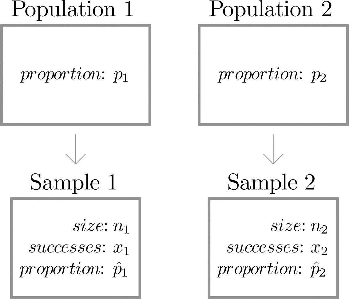
Our goal is to use the information in the samples to estimate the difference $p_{1} - p_{2}$ in the two population proportions and to make statistically valid inferences about it.

Confidence Intervals

Since the sample proportion ${\hat{p}}_{1}$ computed using the sample drawn from Population 1 is a good estimator of population proportion p₁ of Population 1 and the sample proportion ${\hat{p}}_{2}$ computed using the sample drawn from Population 2 is a good estimator of population proportion p₂ of Population 2, a reasonable point estimate of the difference $p_{1} - p_{2}$ is ${\hat{p}}_{1} - {\hat{p}}_{2} .$ In order to widen this point estimate into a confidence interval we suppose that both samples are large, as described in Section 7.3 "Large Sample Estimation of a Population Proportion" in Chapter 7 "Estimation" and repeated below. If so, then the following formula for a confidence interval for $p_{1} - p_{2}$ is valid.

$100 (1 - α) %$ Confidence Interval for the Difference Between Two Population Proportions

({\hat{p}}_{1} - {\hat{p}}_{2}) \pm z_{α ∕ 2} \sqrt{\frac{{\hat{p}}_{1} (1 - {\hat{p}}_{1})}{n_{1}} + \frac{{\hat{p}}_{2} (1 - {\hat{p}}_{2})}{n_{2}}}

The samples must be independent, and each sample must be large: each of the intervals

[{\hat{p}}_{1} - 3 \sqrt{\frac{{\hat{p}}_{1} (1 - {\hat{p}}_{1})}{n_{1}}}, {\hat{p}}_{1} + 3 \sqrt{\frac{{\hat{p}}_{1} (1 - {\hat{p}}_{1})}{n_{1}}}]

and

[{\hat{p}}_{2} - 3 \sqrt{\frac{{\hat{p}}_{2} (1 - {\hat{p}}_{2})}{n_{2}}}, {\hat{p}}_{2} + 3 \sqrt{\frac{{\hat{p}}_{2} (1 - {\hat{p}}_{2})}{n_{2}}}]

must lie wholly within the interval $[0,1] .$

Example 10

The department of code enforcement of a county government issues permits to general contractors to work on residential projects. For each permit issued, the department inspects the result of the project and gives a “pass” or “fail” rating. A failed project must be re-inspected until it receives a pass rating. The department had been frustrated by the high cost of re-inspection and decided to publish the inspection records of all contractors on the web. It was hoped that public access to the records would lower the re-inspection rate. A year after the web access was made public, two samples of records were randomly selected. One sample was selected from the pool of records before the web publication and one after. The proportion of projects that passed on the first inspection was noted for each sample. The results are summarized below. Construct a point estimate and a 90% confidence interval for the difference in the passing rate on first inspection between the two time periods.

\begin{array}{l} No public web access & n_{1} = 500 & {\hat{p}}_{1} = 0.67 \\ Public web access & n_{2} = 100 & {\hat{p}}_{2} = 0.80 \end{array}

Solution:

The point estimate of $p_{1} - p_{2}$ is

{\hat{p}}_{1} - {\hat{p}}_{2} = 0.67 - 0.80 = − 0.13

Because the “No public web access” population was labeled as Population 1 and the “Public web access” population was labeled as Population 2, in words this means that we estimate that the proportion of projects that passed on the first inspection increased by 13 percentage points after records were posted on the web.

The sample sizes are sufficiently large for constructing a confidence interval since for sample 1:

3 \sqrt{\frac{{\hat{p}}_{1} (1 - {\hat{p}}_{1})}{n_{1}}} = 3 \sqrt{\frac{(0.67) (0.33)}{500}} = 0.06

so that

\begin{matrix} [{\hat{p}}_{1} − 3 \sqrt{\frac{{\hat{p}}_{1} (1 - {\hat{p}}_{1})}{n_{1}}}, {\hat{p}}_{1} + 3 \sqrt{\frac{{\hat{p}}_{1} (1 - {\hat{p}}_{1})}{n_{1}}}] \\ = [0.67 - 0 . 06,0 . 67 + 0.06] = [0 . 61,0 . 73] \subset [0,1] \end{matrix}

and for sample 2:

3 \sqrt{\frac{{\hat{p}}_{1} (1 - {\hat{p}}_{1})}{n_{1}}} = 3 \sqrt{\frac{(0.8) (0.2)}{100}} = 0.12

so that

\begin{matrix} [{\hat{p}}_{2} − 3 \sqrt{\frac{{\hat{p}}_{2} (1 - {\hat{p}}_{2})}{n_{2}}}, {\hat{p}}_{2} + 3 \sqrt{\frac{{\hat{p}}_{2} (1 - {\hat{p}}_{2})}{n_{2}}}] \\ = [0.8 - 0 . 12,0 . 8 + 0.12] = [0 . 68,0 . 92] \subset [0,1] \end{matrix}

To apply the formula for the confidence interval, we first observe that the 90% confidence level means that $α = 1 - 0.90 = 0.10$ so that $z_{α ∕ 2} = z_{0.05} .$ From Figure 12.3 "Critical Values of " we read directly that $z_{0.05} = 1.645 .$ Thus the desired confidence interval is

\begin{matrix} ({\hat{p}}_{1} - {\hat{p}}_{2}) & \pm & z_{α ∕ 2} \sqrt{\frac{{\hat{p}}_{1} (1 - {\hat{p}}_{1})}{n_{1}} + \frac{{\hat{p}}_{2} (1 - {\hat{p}}_{2})}{n_{2}}} \\ = & − 0.13 \pm 1.645 \sqrt{\frac{(0.67) (0.33)}{500} + \frac{(0.8) (0.2)}{100}} \\ = & − 0.13 \pm 0.07 \end{matrix}

The 90% confidence interval is $[− 0.20, − 0.06] .$ We are 90% confident that the difference in the population proportions lies in the interval $[− 0.20, − 0.06]$ , in the sense that in repeated sampling 90% of all intervals constructed from the sample data in this manner will contain $p_{1} - p_{2} .$ Taking into account the labeling of the two populations, this means that we are 90% confident that the proportion of projects that pass on the first inspection is between 6 and 20 percentage points higher after public access to the records than before.

Hypothesis Testing

In hypothesis tests concerning the relative sizes of the proportions p₁ and p₂ of two populations that possess a particular characteristic, the null and alternative hypotheses will always be expressed in terms of the difference of the two population proportions. Hence the null hypothesis is always written

H_{0} : p_{1} - p_{2} = D_{0}

The three forms of the alternative hypothesis, with the terminology for each case, are:

Form of $H_{a}$	Terminology
$H_{a} : p_{1} - p_{2} < D_{0}$	Left-tailed
$H_{a} : p_{1} - p_{2} > D_{0}$	Right-tailed
$H_{a} : p_{1} - p_{2} \neq D_{0}$	Two-tailed

As long as the samples are independent and both are large the following formula for the standardized test statistic is valid, and it has the standard normal distribution.

Standardized Test Statistic for Hypothesis Tests Concerning the Difference Between Two Population Proportions

Z = \frac{({\hat{p}}_{1} - {\hat{p}}_{2}) - D_{0}}{\sqrt{\frac{{\hat{p}}_{1} (1 - {\hat{p}}_{1})}{n_{1}} + \frac{{\hat{p}}_{2} (1 - {\hat{p}}_{2})}{n_{2}}}}

The test statistic has the standard normal distribution.

The samples must be independent, and each sample must be large: each of the intervals

[{\hat{p}}_{1} - 3 \sqrt{\frac{{\hat{p}}_{1} (1 - {\hat{p}}_{1})}{n_{1}}}, {\hat{p}}_{1} + 3 \sqrt{\frac{{\hat{p}}_{1} (1 - {\hat{p}}_{1})}{n_{1}}}]

and

[{\hat{p}}_{2} - 3 \sqrt{\frac{{\hat{p}}_{2} (1 - {\hat{p}}_{2})}{n_{2}}}, {\hat{p}}_{2} + 3 \sqrt{\frac{{\hat{p}}_{2} (1 - {\hat{p}}_{2})}{n_{2}}}]

must lie wholly within the interval $[0,1] .$

Example 11

Using the data of Note 9.25 "Example 10", test whether there is sufficient evidence to conclude that public web access to the inspection records has increased the proportion of projects that passed on the first inspection by more than 5 percentage points. Use the critical value approach at the 10% level of significance.

Solution:

Step 1. Taking into account the labeling of the populations an increase in passing rate at the first inspection by more than 5 percentage points after public access on the web may be expressed as $p_{2} > p_{1} + 0.05$ , which by algebra is the same as $p_{1} - p_{2} < − 0.05 .$ This is the alternative hypothesis. Since the null hypothesis is always expressed as an equality, with the same number on the right as is in the alternative hypothesis, the test is
$\begin{matrix} H_{0} : p_{1} - p_{2} & = & − 0.05 \\ vs. H_{a} : p_{1} - p_{2} & < & − 0.05 & @ α = 0.10 \end{matrix}$
Step 2. Since the test is with respect to a difference in population proportions the test statistic is
$Z = \frac{({\hat{p}}_{1} - {\hat{p}}_{2}) - D_{0}}{\sqrt{\frac{{\hat{p}}_{1} (1 - {\hat{p}}_{1})}{n_{1}} + \frac{{\hat{p}}_{2} (1 - {\hat{p}}_{2})}{n_{2}}}}$
Step 3. Inserting the values given in Note 9.25 "Example 10" and the value $D_{0} = − 0.05$ into the formula for the test statistic gives
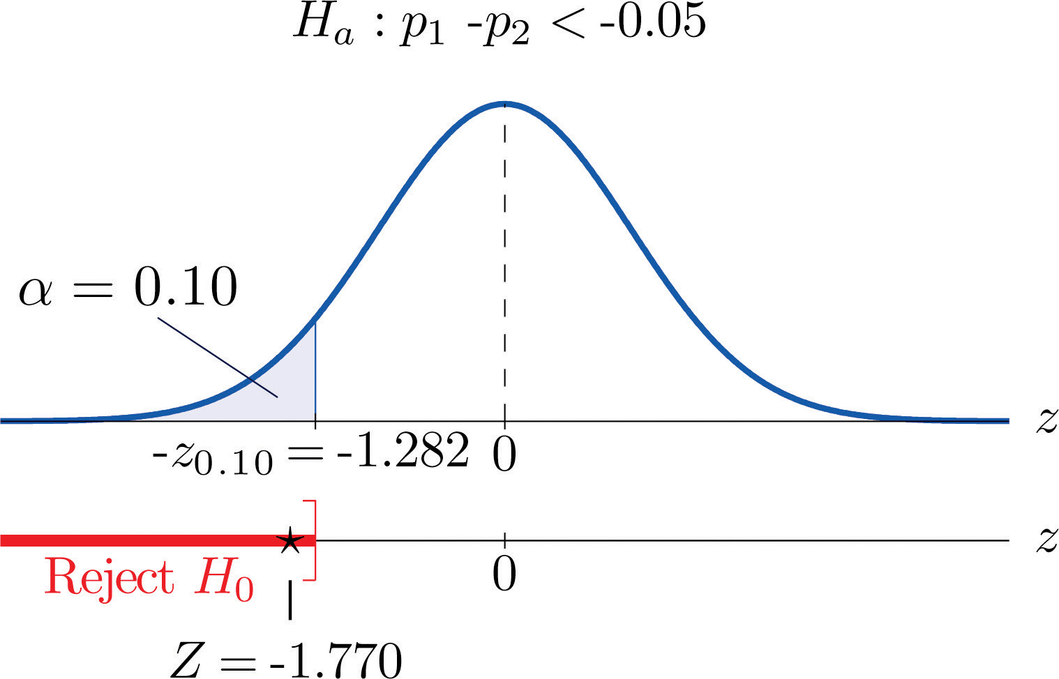
$Z = \frac{({\hat{p}}_{1} - {\hat{p}}_{2}) - D_{0}}{\sqrt{\frac{{\hat{p}}_{1} (1 - {\hat{p}}_{1})}{n_{1}} + \frac{{\hat{p}}_{2} (1 - {\hat{p}}_{2})}{n_{2}}}} = \frac{(− 0.13) - (− 0.05)}{\sqrt{\frac{(0.67) (0.33)}{500} + \frac{(0.8) (0.2)}{100}}} = − 1.770$
Step 4. Since the symbol in H_a is “<” this is a left-tailed test, so there is a single critical value, $z_{α} = − z_{0.10} .$ From the last row in Figure 12.3 "Critical Values of " $z_{0.10} = 1.282$ , so $− z_{0.10} = − 1.282 .$ The rejection region is $(− \infty, − 1.282] .$
Step 5. As shown in Figure 9.8 "Rejection Region and Test Statistic for " the test statistic falls in the rejection region. The decision is to reject H₀. In the context of the problem our conclusion is:

The data provide sufficient evidence, at the 10% level of significance, to conclude that the rate of passing on the first inspection has increased by more than 5 percentage points since records were publicly posted on the web.

Figure 9.8 Rejection Region and Test Statistic for Note 9.27 "Example 11"

Example 12

Perform the test of Note 9.27 "Example 11" using the p-value approach.

Solution:

The first three steps are identical to those in Note 9.27 "Example 11".

Step 4. Because the test is left-tailed the observed significance or p-value of the test is just the area of the left tail of the standard normal distribution that is cut off by the test statistic $Z = − 1.770 .$ From Figure 12.2 "Cumulative Normal Probability" the area of the left tail determined by −1.77 is 0.0384. The p-value is 0.0384.
Step 5. Since the p-value 0.0384 is less than $α = 0.10$ , the decision is to reject the null hypothesis: The data provide sufficient evidence, at the 10% level of significance, to conclude that the rate of passing on the first inspection has increased by more than 5 percentage points since records were publicly posted on the web.

Finally a common misuse of the formulas given in this section must be mentioned. Suppose a large pre-election survey of potential voters is conducted. Each person surveyed is asked to express a preference between, say, Candidate A and Candidate B. (Perhaps “no preference” or “other” are also choices, but that is not important.) In such a survey, estimators ${\hat{p}}_{A}$ and ${\hat{p}}_{B}$ of p_A and p_B can be calculated. It is important to realize, however, that these two estimators were not calculated from two independent samples. While ${\hat{p}}_{A} - {\hat{p}}_{B}$ may be a reasonable estimator of $p_{A} - p_{B}$ , the formulas for confidence intervals and for the standardized test statistic given in this section are not valid for data obtained in this manner.

Key Takeaways

A confidence interval for the difference in two population proportions is computed using a formula in the same fashion as was done for a single population mean.
The same five-step procedure used to test hypotheses concerning a single population proportion is used to test hypotheses concerning the difference between two population proportions. The only difference is in the formula for the standardized test statistic.

Exercises

Basic

Construct the confidence interval for $p_{1} - p_{2}$ for the level of confidence and the data given. (The samples are sufficiently large.)
1. 90% confidence,
  
  $n_{1} = 1670$ , ${\hat{p}}_{1} = 0.42$
  
  $n_{2} = 900$ , ${\hat{p}}_{2} = 0.38$
2. 95% confidence,
  
  $n_{1} = 600$ , ${\hat{p}}_{1} = 0.84$
  
  $n_{2} = 420$ , ${\hat{p}}_{2} = 0.67$
Construct the confidence interval for $p_{1} - p_{2}$ for the level of confidence and the data given. (The samples are sufficiently large.)
1. 98% confidence,
  
  $n_{1} = 750$ , ${\hat{p}}_{1} = 0.64$
  
  $n_{2} = 800$ , ${\hat{p}}_{2} = 0.51$
2. 99.5% confidence,
  
  $n_{1} = 250$ , ${\hat{p}}_{1} = 0.78$
  
  $n_{2} = 250$ , ${\hat{p}}_{2} = 0.51$
Construct the confidence interval for $p_{1} - p_{2}$ for the level of confidence and the data given. (The samples are sufficiently large.)
1. 80% confidence,
  
  $n_{1} = 300$ , ${\hat{p}}_{1} = 0.255$
  
  $n_{2} = 400$ , ${\hat{p}}_{2} = 0.193$
2. 95% confidence,
  
  $n_{1} = 3500$ , ${\hat{p}}_{1} = 0.147$
  
  $n_{2} = 3750$ , ${\hat{p}}_{2} = 0.131$
Construct the confidence interval for $p_{1} - p_{2}$ for the level of confidence and the data given. (The samples are sufficiently large.)
1. 99% confidence,
  
  $n_{1} = 2250$ , ${\hat{p}}_{1} = 0.915$
  
  $n_{2} = 2525$ , ${\hat{p}}_{2} = 0.858$
2. 95% confidence,
  
  $n_{1} = 120$ , ${\hat{p}}_{1} = 0.650$
  
  $n_{2} = 200$ , ${\hat{p}}_{2} = 0.505$
Perform the test of hypotheses indicated, using the data given. Use the critical value approach. Compute the p-value of the test as well. (The samples are sufficiently large.)
1. Test $H_{0} : p_{1} - p_{2} = 0$ vs. $H_{a} : p_{1} - p_{2} > 0$ @ $α = 0.10$ ,
  
  $n_{1} = 1200$ , ${\hat{p}}_{1} = 0.42$
  
  $n_{2} = 1200$ , ${\hat{p}}_{2} = 0.40$
2. Test $H_{0} : p_{1} - p_{2} = 0$ vs. $H_{a} : p_{1} - p_{2} \neq 0$ @ $α = 0.05$ ,
  
  $n_{1} = 550$ , ${\hat{p}}_{1} = 0.61$
  
  $n_{2} = 600$ , ${\hat{p}}_{2} = 0.67$
Perform the test of hypotheses indicated, using the data given. Use the critical value approach. Compute the p-value of the test as well. (The samples are sufficiently large.)
1. Test $H_{0} : p_{1} - p_{2} = 0.05$ vs. $H_{a} : p_{1} - p_{2} > 0.05$ @ $α = 0.05$ ,
  
  $n_{1} = 1100$ , ${\hat{p}}_{1} = 0.57$
  
  $n_{2} = 1100$ , ${\hat{p}}_{2} = 0.48$
2. Test $H_{0} : p_{1} - p_{2} = 0$ vs. $H_{a} : p_{1} - p_{2} \neq 0$ @ $α = 0.05$ ,
  
  $n_{1} = 800$ , ${\hat{p}}_{1} = 0.39$
  
  $n_{2} = 900$ , ${\hat{p}}_{2} = 0.43$
Perform the test of hypotheses indicated, using the data given. Use the critical value approach. Compute the p-value of the test as well. (The samples are sufficiently large.)
1. Test $H_{0} : p_{1} - p_{2} = 0.25$ vs. $H_{a} : p_{1} - p_{2} < 0.25$ @ $α = 0.005$ ,
  
  $n_{1} = 1400$ , ${\hat{p}}_{1} = 0.57$
  
  $n_{2} = 1200$ , ${\hat{p}}_{2} = 0.37$
2. Test $H_{0} : p_{1} - p_{2} = 0.16$ vs. $H_{a} : p_{1} - p_{2} \neq 0.16$ @ $α = 0.02$ ,
  
  $n_{1} = 750$ , ${\hat{p}}_{1} = 0.43$
  
  $n_{2} = 600$ , ${\hat{p}}_{2} = 0.22$
Perform the test of hypotheses indicated, using the data given. Use the critical value approach. Compute the p-value of the test as well. (The samples are sufficiently large.)
1. Test $H_{0} : p_{1} - p_{2} = 0.08$ vs. $H_{a} : p_{1} - p_{2} > 0.08$ @ $α = 0.025$ ,
  
  $n_{1} = 450$ , ${\hat{p}}_{1} = 0.67$
  
  $n_{2} = 200$ , ${\hat{p}}_{2} = 0.52$
2. Test $H_{0} : p_{1} - p_{2} = 0.02$ vs. $H_{a} : p_{1} - p_{2} \neq 0.02$ @ $α = 0.001$ ,
  
  $n_{1} = 2700$ , ${\hat{p}}_{1} = 0.837$
  
  $n_{2} = 2900$ , ${\hat{p}}_{2} = 0.854$
Perform the test of hypotheses indicated, using the data given. Use the p-value approach. (The samples are sufficiently large.)
1. Test $H_{0} : p_{1} - p_{2} = 0$ vs. $H_{a} : p_{1} - p_{2} < 0$ @ $α = 0.005$ ,
  
  $n_{1} = 1100$ , ${\hat{p}}_{1} = 0.22$
  
  $n_{2} = 1300$ , ${\hat{p}}_{2} = 0.27$
2. Test $H_{0} : p_{1} - p_{2} = 0$ vs. $H_{a} : p_{1} - p_{2} \neq 0$ @ $α = 0.01$ ,
  
  $n_{1} = 650$ , ${\hat{p}}_{1} = 0.35$
  
  $n_{2} = 650$ , ${\hat{p}}_{2} = 0.41$
Perform the test of hypotheses indicated, using the data given. Use the p-value approach. (The samples are sufficiently large.)
1. Test $H_{0} : p_{1} - p_{2} = 0.15$ vs. $H_{a} : p_{1} - p_{2} > 0.15$ @ $α = 0.10$ ,
  
  $n_{1} = 950$ , ${\hat{p}}_{1} = 0.41$
  
  $n_{2} = 500$ , ${\hat{p}}_{2} = 0.23$
2. Test $H_{0} : p_{1} - p_{2} = 0.10$ vs. $H_{a} : p_{1} - p_{2} \neq 0.10$ @ $α = 0.10$ ,
  
  $n_{1} = 220$ , ${\hat{p}}_{1} = 0.92$
  
  $n_{2} = 160$ , ${\hat{p}}_{2} = 0.78$
Perform the test of hypotheses indicated, using the data given. Use the p-value approach. (The samples are sufficiently large.)
1. Test $H_{0} : p_{1} - p_{2} = 0.22$ vs. $H_{a} : p_{1} - p_{2} > 0.22$ @ $α = 0.05$ ,
  
  $n_{1} = 90$ , ${\hat{p}}_{1} = 0.72$
  
  $n_{2} = 75$ , ${\hat{p}}_{2} = 0.40$
2. Test $H_{0} : p_{1} - p_{2} = 0.37$ vs. $H_{a} : p_{1} - p_{2} \neq 0.37$ @ $α = 0.02$ ,
  
  $n_{1} = 425$ , ${\hat{p}}_{1} = 0.772$
  
  $n_{2} = 425$ , ${\hat{p}}_{2} = 0.331$
Perform the test of hypotheses indicated, using the data given. Use the p-value approach. (The samples are sufficiently large.)
1. Test $H_{0} : p_{1} - p_{2} = 0.50$ vs. $H_{a} : p_{1} - p_{2} < 0.50$ @ $α = 0.10$ ,
  
  $n_{1} = 40$ , ${\hat{p}}_{1} = 0.65$
  
  $n_{2} = 55$ , ${\hat{p}}_{2} = 0.24$
2. Test $H_{0} : p_{1} - p_{2} = 0.30$ vs. $H_{a} : p_{1} - p_{2} \neq 0.30$ @ $α = 0.10$ ,
  
  $n_{1} = 7500$ , ${\hat{p}}_{1} = 0.664$
  
  $n_{2} = 1000$ , ${\hat{p}}_{2} = 0.319$

Applications

In all the remaining exercsises the samples are sufficiently large (so this need not be checked).

Voters in a particular city who identify themselves with one or the other of two political parties were randomly selected and asked if they favor a proposal to allow citizens with proper license to carry a concealed handgun in city parks. The results are:

	Party A	Party B
Sample size, n	150	200
Number in favor, x	90	140

Give a point estimate for the difference in the proportion of all members of Party A and all members of Party B who favor the proposal.
Construct the 95% confidence interval for the difference, based on these data.
Test, at the 5% level of significance, the hypothesis that the proportion of all members of Party A who favor the proposal is less than the proportion of all members of Party B who do.
Compute the p-value of the test.

To investigate a possible relation between gender and handedness, a random sample of 320 adults was taken, with the following results:

	Men	Women
Sample size, n	168	152
Number of left-handed, x	24	9

Give a point estimate for the difference in the proportion of all men who are left-handed and the proportion of all women who are left-handed.
Construct the 95% confidence interval for the difference, based on these data.
Test, at the 5% level of significance, the hypothesis that the proportion of men who are left-handed is greater than the proportion of women who are.
Compute the p-value of the test.

A local school board member randomly sampled private and public high school teachers in his district to compare the proportions of National Board Certified (NBC) teachers in the faculty. The results were:

	Private Schools	Public Schools
Sample size, n	80	520
Proportion of NBC teachers, $\hat{p}$	0.175	0.150

Give a point estimate for the difference in the proportion of all teachers in area public schools and the proportion of all teachers in private schools who are National Board Certified.
Construct the 90% confidence interval for the difference, based on these data.
Test, at the 10% level of significance, the hypothesis that the proportion of all public school teachers who are National Board Certified is less than the proportion of private school teachers who are.
Compute the p-value of the test.

In professional basketball games, the fans of the home team always try to distract free throw shooters on the visiting team. To investigate whether this tactic is actually effective, the free throw statistics of a professional basketball player with a high free throw percentage were examined. During the entire last season, this player had 656 free throws, 420 in home games and 236 in away games. The results are summarized below.

	Home	Away
Sample size, n	420	236
Free throw percent, $\hat{p}$	81.5%	78.8%

Give a point estimate for the difference in the proportion of free throws made at home and away.
Construct the 90% confidence interval for the difference, based on these data.
Test, at the 10% level of significance, the hypothesis that there exists a home advantage in free throws.
Compute the p-value of the test.

Randomly selected middle-aged people in both China and the United States were asked if they believed that adults have an obligation to financially support their aged parents. The results are summarized below.

	China	USA
Sample size, n	1300	150
Number of yes, x	1170	110

Test, at the 1% level of significance, whether the data provide sufficient evidence to conclude that there exists a cultural difference in attitude regarding this question.

A manufacturer of walk-behind push mowers receives refurbished small engines from two new suppliers, A and B. It is not uncommon that some of the refurbished engines need to be lightly serviced before they can be fitted into mowers. The mower manufacturer recently received 100 engines from each supplier. In the shipment from A, 13 needed further service. In the shipment from B, 10 needed further service. Test, at the 10% level of significance, whether the data provide sufficient evidence to conclude that there exists a difference in the proportions of engines from the two suppliers needing service.

Large Data Set Exercises

Large Data Sets 6A and 6B record results of a random survey of 200 voters in each of two regions, in which they were asked to express whether they prefer Candidate A for a U.S. Senate seat or prefer some other candidate. Let the population of all voters in region 1 be denoted Population 1 and the population of all voters in region 2 be denoted Population 2. Let p₁ be the proportion of voters in Population 1 who prefer Candidate A, and p₂ the proportion in Population 2 who do.

http://www.gone.2012books.lardbucket.org/sites/all/files/data6A.xls

http://www.gone.2012books.lardbucket.org/sites/all/files/data6B.xls
1. Find the relevant sample proportions ${\hat{p}}_{1}$ and ${\hat{p}}_{2} .$
2. Construct a point estimate for $p_{1} - p_{2} .$
3. Construct a 95% confidence interval for $p_{1} - p_{2} .$
4. Test, at the 5% level of significance, the hypothesis that the same proportion of voters in the two regions favor Candidate A, against the alternative that a larger proportion in Population 2 do.
Large Data Set 11 records the results of samples of real estate sales in a certain region in the year 2008 (lines 2 through 536) and in the year 2010 (lines 537 through 1106). Foreclosure sales are identified with a 1 in the second column. Let all real estate sales in the region in 2008 be Population 1 and all real estate sales in the region in 2010 be Population 2.

http://www.gone.2012books.lardbucket.org/sites/all/files/data11.xls
1. Use the sample data to construct point estimates ${\hat{p}}_{1}$ and ${\hat{p}}_{2}$ of the proportions p₁ and p₂ of all real estate sales in this region in 2008 and 2010 that were foreclosure sales. Construct a point estimate of $p_{1} - p_{2} .$
2. Use the sample data to construct a 90% confidence for $p_{1} - p_{2} .$
3. Test, at the 10% level of significance, the hypothesis that the proportion of real estate sales in the region in 2010 that were foreclosure sales was greater than the proportion of real estate sales in the region in 2008 that were foreclosure sales. (The default is that the proportions were the same.)

Answers

1. $(0 . 0068,0 . 0732)$ ,
2. $(0 . 1163,0 . 2237)$
1. $(0 . 0210,0 . 1030)$ ,
2. $(0 . 0001,0 . 0319)$
1. Z = 0.996, $z_{0.10} = 1.282$ , $p -value = 0.1587$ , do not reject H₀,
2. $Z = − 2.120$ , $\pm z_{0.025} = \pm 1.960$ , $p -value = 0.0340$ , reject H₀
1. $Z = − 2.602$ , $− z_{0.005} = − 2.576$ , $p -value = 0.0047$ , reject H₀,
2. Z = 2.020, $\pm z_{0.01} = \pm 2.326$ , $p -value = 0.0434$ , do not reject H₀
1. $Z = − 2.85$ , $p -value = 0.0022$ , reject H₀,
2. $Z = − 2.23$ , $p -value = 0.0258$ , do not reject H₀
1. Z = 1.36, $p -value = 0.0869$ , do not reject H₀,
2. Z = 2.32, $p -value = 0.0204$ , do not reject H₀

1. −0.10,
2. $− 0.10 \pm 0.101$ ,
3. $Z = − 1.943$ , $− z_{0.05} = − 1.645$ , reject H₀ (fewer in Party A favor),
4. p-value = 0.0262
1. 0.025,
2. $0.025 \pm 0.0745$ ,
3. Z = 0.552, $z_{0.10} = 1.282$ , do not reject H₀ (as many public school teachers are certified),
4. p-value = 0.2912
Z = 4.498, $\pm z_{0.005} = \pm 2.576$ , reject H₀ (different)

1. ${\hat{p}}_{1} = 0.355$ and ${\hat{p}}_{2} = 0.41$
2. ${\hat{p}}_{1} - {\hat{p}}_{2} = − 0.055$
3. $(− 0 . 1501,0 . 0401)$
4. $H_{0} : p_{1} - p_{2} = 0$ vs. $H_{a} : p_{1} - p_{2} < 0 .$ Test Statistic: $Z = − 1.1335 .$ Rejection Region: $(− \infty, − 1.645] .$ Decision: Fail to reject H₀.

9.4 Comparison of Two Population Proportions

Learning Objectives

Confidence Intervals

100(1−α)% Confidence Interval for the Difference Between Two Population Proportions

Example 10

Hypothesis Testing

Standardized Test Statistic for Hypothesis Tests Concerning the Difference Between Two Population Proportions

Example 11

Example 12

Key Takeaways

Exercises

Basic

Applications

Large Data Set Exercises

Answers

$100 (1 - α) %$ Confidence Interval for the Difference Between Two Population Proportions