Question: Recall the conversation that Eric (CFO) and Susan (cost accountant) had about Bikes Unlimited’s budget for the next month, which is August. The company expects to increase sales by 10 to 20 percent, and Susan has been asked to estimate profit for August given this expected increase. Although examples of variable and fixed costs were provided in the previous sections, companies typically do not know exactly how much of their costs are fixed and how much are variable. (Financial accounting systems do not normally sort costs as fixed or variable.) Thus organizations must estimate their fixed and variable costs. What methods do organizations use to estimate fixed and variable costs?
Answer: Four common approaches are used to estimate fixed and variable costs:
All four methods are described next. The goal of each cost estimation method is to estimate fixed and variable costs and to describe this estimate in the form of Y = f + vX. That is, Total mixed cost = Total fixed cost + (Unit variable cost × Number of units). Note that the estimates presented next for Bikes Unlimited may differ from the dollar amounts used previously, which were for illustrative purposes only.
Question: The account analysisA method of cost analysis that requires a review of accounts by an experienced employee or group of employees to determine whether the costs in each account are fixed or variable. approach is perhaps the most common starting point for estimating fixed and variable costs. How is the account analysis approach used to estimate fixed and variable costs?
Answer: This approach requires that an experienced employee or group of employees review the appropriate accounts and determine whether the costs in each account are fixed or variable. Totaling all costs identified as fixed provides the estimate of total fixed costs. To determine the variable cost per unit, all costs identified as variable are totaled and divided by the measure of activity (units produced is the measure of activity for Bikes Unlimited).
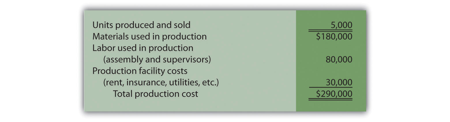
Let’s look at the account analysis approach using Bikes Unlimited as an example. Susan (the cost accountant) asked the financial accounting department to provide cost information for the production department for the month of June (July information is not yet available). Because the financial accounting department tracks information by department, it is able to produce this information. The production department information for June is as follows:
Susan reviewed this cost information with the production manager, Indira Bingham, who has worked as production manager at Bikes Unlimited for several years. After careful review, Indira and Susan came up with the following breakdown of variable and fixed costs for June:
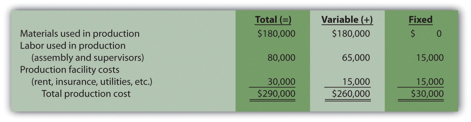
Total fixed cost is estimated to be $30,000, and variable cost per unit is estimated to be $52 (= $260,000 ÷ 5,000 units produced). Remember, the goal is to describe the mixed costs in the equation form Y = f + vX. Thus the mixed cost equation used to estimate future production costs is
Y = $30,000 + $52XNow Susan can estimate monthly production costs (Y) if she knows how many units Bikes Unlimited plans to produce (X). For example, if Bikes Unlimited plans to produce 6,000 units for a particular month (a 20 percent increase over June) and this level of activity is within the relevant range, total production costs should be approximately $342,000 [= $30,000 + ($52 × 6,000 units)].
Question: Why should Susan be careful using historical data for one month (June) to estimate future costs?
Answer: June may not be a typical month for Bikes Unlimited. For example, utility costs may be low relative to those in the winter months, and production costs may be relatively high as the company prepares for increased demand in July and August. This might result in a lower materials cost per unit from quantity discounts offered by suppliers. To smooth out these fluctuations, companies often use data from the past quarter or past year to estimate costs.
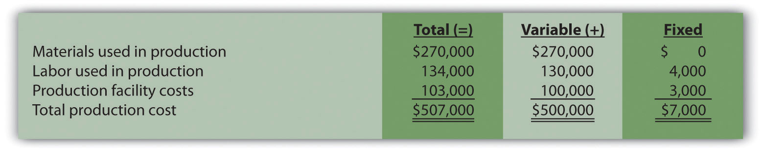
Alta Production, Inc., is using the account analysis approach to identify the behavior of production costs for a month in which it produced 350 units. The production manager was asked to review these costs and provide her best guess as to how they should be categorized. She responded with the following information:
Solution to Review Problem 5.2
Using the previous equation, simply substitute 400 units for X, as follows:
Thus total production costs are expected to be $578,428 for next month.
Question: Another approach to identifying fixed and variable costs for cost estimation purposes is the high-low methodA method of cost analysis that uses the high and low activity data points to estimate fixed and variable costs.. Accountants who use this approach are looking for a quick and easy way to estimate costs, and will follow up their analysis with other more accurate techniques. How is the high-low method used to estimate fixed and variable costs?
Answer: The high-low method uses historical information from several reporting periods to estimate costs. Assume Susan Wesley obtains monthly production cost information from the financial accounting department for the last 12 months. This information appears in Table 5.4 "Monthly Production Costs for Bikes Unlimited".
Table 5.4 Monthly Production Costs for Bikes Unlimited
| Reporting Period (Month) | Total Production Costs | Level of Activity (Units Produced) |
|---|---|---|
| July | $230,000 | 3,500 |
| August | 250,000 | 3,750 |
| September | 260,000 | 3,800 |
| October | 220,000 | 3,400 |
| November | 340,000 | 5,800 |
| December | 330,000 | 5,500 |
| January | 200,000 | 2,900 |
| February | 210,000 | 3,300 |
| March | 240,000 | 3,600 |
| April | 380,000 | 5,900 |
| May | 350,000 | 5,600 |
| June | 290,000 | 5,000 |
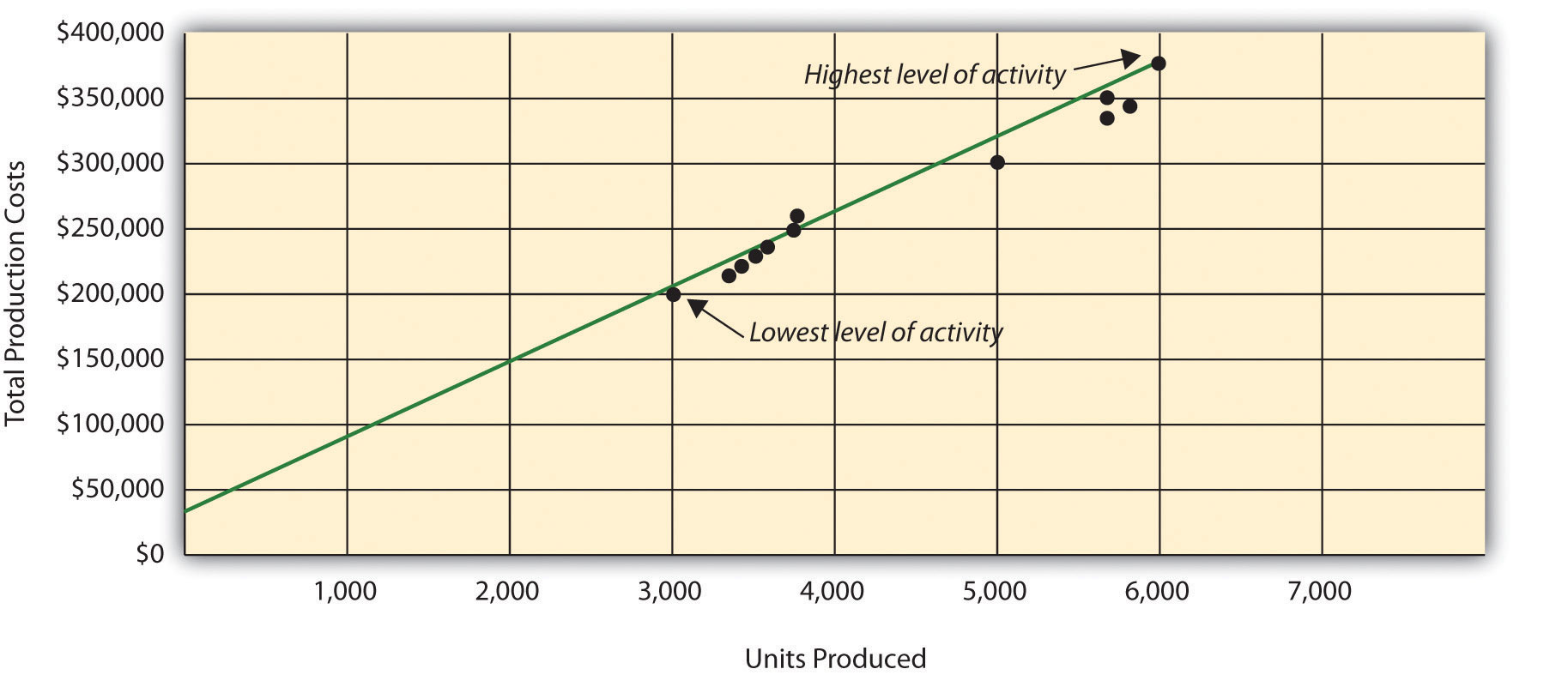
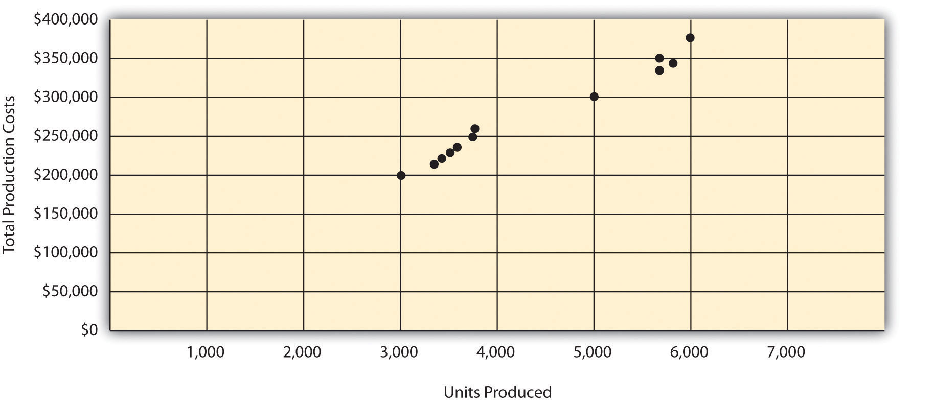
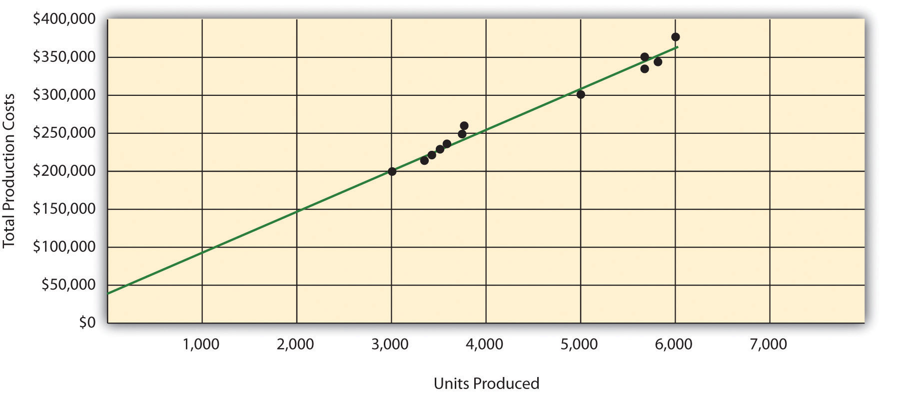
All of the data points from Table 5.4 "Monthly Production Costs for Bikes Unlimited" are plotted on the graph shown in Figure 5.4 "Estimated Total Mixed Production Costs for Bikes Unlimited: High-Low Method". Although a graph is not required using the high-low method, it is a helpful visual tool. Susan then draws a straight line using the high (April) and low (January) activity levels from these data. The goal of the high-low method is to describe this line mathematically in the form of an equation stated as Y = f + vX, which requires calculating both the total fixed costs amount (f) and per unit variable cost amount (v). Four steps are required to achieve this using the high-low method:
Step 1. Identify the high and low activity levels from the data set.
Step 2. Calculate the variable cost per unit (v).
Step 3. Calculate the total fixed cost (f).
Step 4. State the results in equation form Y = f + vX.
Figure 5.4 Estimated Total Mixed Production Costs for Bikes Unlimited: High-Low Method
Question: How are the four steps of the high-low method used to estimate total fixed costs and per unit variable cost?
Answer: Each of the four steps is described next.
Step 1. Identify the high and low activity levels from the data set.
The highest level of activity (level of production) occurred in the month of April (5,900 units; $380,000 production costs), and the lowest level of activity occurred in the month of January (2,900 units; $200,000 production costs). Note that we are identifying the high and low activity levels rather than the high and low dollar levels—choosing the high and low dollar levels can result in incorrect high and low points.
Step 2. Calculate the variable cost per unit (v).
Because the slope of the line shown in Figure 5.4 "Estimated Total Mixed Production Costs for Bikes Unlimited: High-Low Method" represents the variable cost per unit, the goal here is to calculate the slope of the line using the high and low points identified in step 1 (the slope calculation is often referred to as “rise over run” in math courses). The calculation of the variable cost per unit for Bikes Unlimited is shown as follows:
Step 3. Calculate the total fixed cost (f).
After completing step 2, the equation to describe the line is partially complete and stated as Y = f + $60X. The goal of step 3 is to calculate a value for total fixed cost (f). Simply select either the high or low activity level, and fill in the data to solve for f (total fixed costs), as shown.
Using the low activity level of 2,900 units and $200,000,
Thus total fixed costs total $26,000. (Try this using the high activity level of 5,900 units and $380,000. You will get the same result as long as the per unit variable cost is not rounded.)
Step 4. State the results in equation form Y = f + vX.
We know from step 2 that the variable cost per unit is $60, and from step 3 that total fixed cost is $26,000. Thus we can state the equation used to estimate total costs as
Y = $26,000 + $60XNow it is possible to estimate total production costs given a certain level of production (X). For example, if Bikes Unlimited expects to produce 6,000 units during August, total production costs are estimated to be $386,000:
Question: Although the high-low method is relatively simple, it does have a potentially significant weakness. What is the potential weakness in using the high-low method?
Answer: In reviewing Figure 5.4 "Estimated Total Mixed Production Costs for Bikes Unlimited: High-Low Method", you will notice that this approach only considers the high and low activity levels in establishing an estimate of fixed and variable costs. The high and low data points may not represent the data set as a whole, and using these points can result in distorted estimates.
For example, the $380,000 in production costs incurred in April may be higher than normal because several production machines broke down resulting in costly repairs. Or perhaps several key employees left the company, resulting in higher than normal labor costs for the month because the remaining employees were paid overtime. Cost accountants will often throw out the high and low points for this reason and use the next highest and lowest points to perform this analysis. While the high-low method is most often used as a quick and easy way to estimate fixed and variable costs, other more sophisticated methods are most often used to refine the estimates developed from the high-low method.
Alta Production, Inc., reported the following production costs for the 12 months January through December. (This is the same company featured in Note 5.15 "Review Problem 5.2".)
| Reporting Period (Month) | Total Production Costs | Level of Activity (Units Produced) |
| January | $460,000 | 300 |
| February | 300,000 | 220 |
| March | 480,000 | 330 |
| April | 550,000 | 390 |
| May | 570,000 | 410 |
| June | 310,000 | 240 |
| July | 440,000 | 290 |
| August | 455,000 | 320 |
| September | 530,000 | 380 |
| October | 250,000 | 150 |
| November | 700,000 | 450 |
| December | 490,000 | 350 |
Solution to Review Problem 5.3
The four steps are as follows:
Step 1. Identify the high and low activity levels from the data set.
The highest level of activity occurred in November (450 units; $700,000 production costs), and the lowest level of activity occurred in October (150 units; $250,000 production costs).
Step 2. Calculate the variable cost per unit (v).
Step 3. Calculate the total fixed cost (f).
After completing step 2, the equation to describe the line is partially complete and stated as Y = f + $1,500X. To calculate total fixed costs, simply select either the high or low activity level, and fill in the data to solve for f (total fixed costs), as shown.
Using the high activity level,
Thus total fixed cost is $25,000.
Step 4. State the results in equation form Y = f + vX.
We know from step 2 that the variable cost per unit is $1,500, and from step 3 that total fixed costs are $25,000. Thus the equation used to estimate total production costs is
Using the equation from part 1, simply substitute 400 units for X, as follows:
Thus total production costs are expected to be $625,000 for next month.
Question: Many organizations prefer to use the scattergraph methodA method of cost analysis that uses a set of data points to estimate fixed and variable costs. to estimate costs. Accountants who use this approach are looking for an approach that does not simply use the highest and lowest data points. How is the scattergraph method used to estimate fixed and variable costs?
Answer: The scattergraph method considers all data points, not just the highest and lowest levels of activity. Again, the goal is to develop an estimate of fixed and variable costs stated in equation form Y = f + vX. Using the same data for Bikes Unlimited shown in Table 5.4 "Monthly Production Costs for Bikes Unlimited", we will follow the five steps associated with the scattergraph method:
Step 1. Plot the data points for each period on a graph.
Step 2. Visually fit a line to the data points and be sure the line touches one data point.
Step 3. Estimate the total fixed costs (f).
Step 4. Calculate the variable cost per unit (v).
Step 5. State the results in equation form Y = f + vX.
Question: How are the five steps of the scattergraph method used to estimate total fixed costs and per unit variable cost?
Answer: Each of the five steps is described next.
Step 1. Plot the data points for each period on a graph.
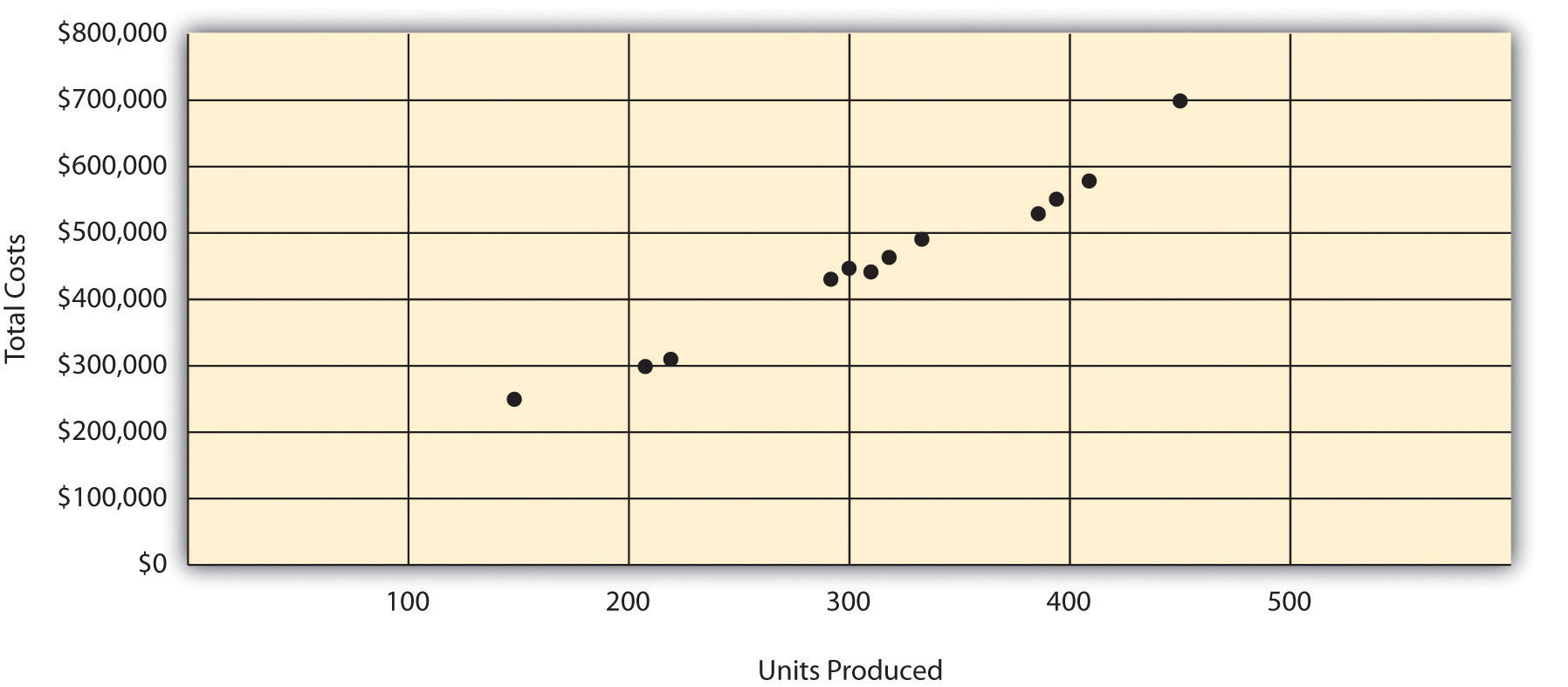
This step requires that each data point be plotted on a graph. The x-axis (horizontal axis) reflects the level of activity (units produced in this example), and the y-axis (vertical axis) reflects the total production cost. Figure 5.5 "Scattergraph of Total Mixed Production Costs for Bikes Unlimited" shows a scattergraph for Bikes Unlimited using the data points for 12 months, July through June.
Figure 5.5 Scattergraph of Total Mixed Production Costs for Bikes Unlimited
Step 2. Visually fit a line to the data points and be sure the line touches one data point.
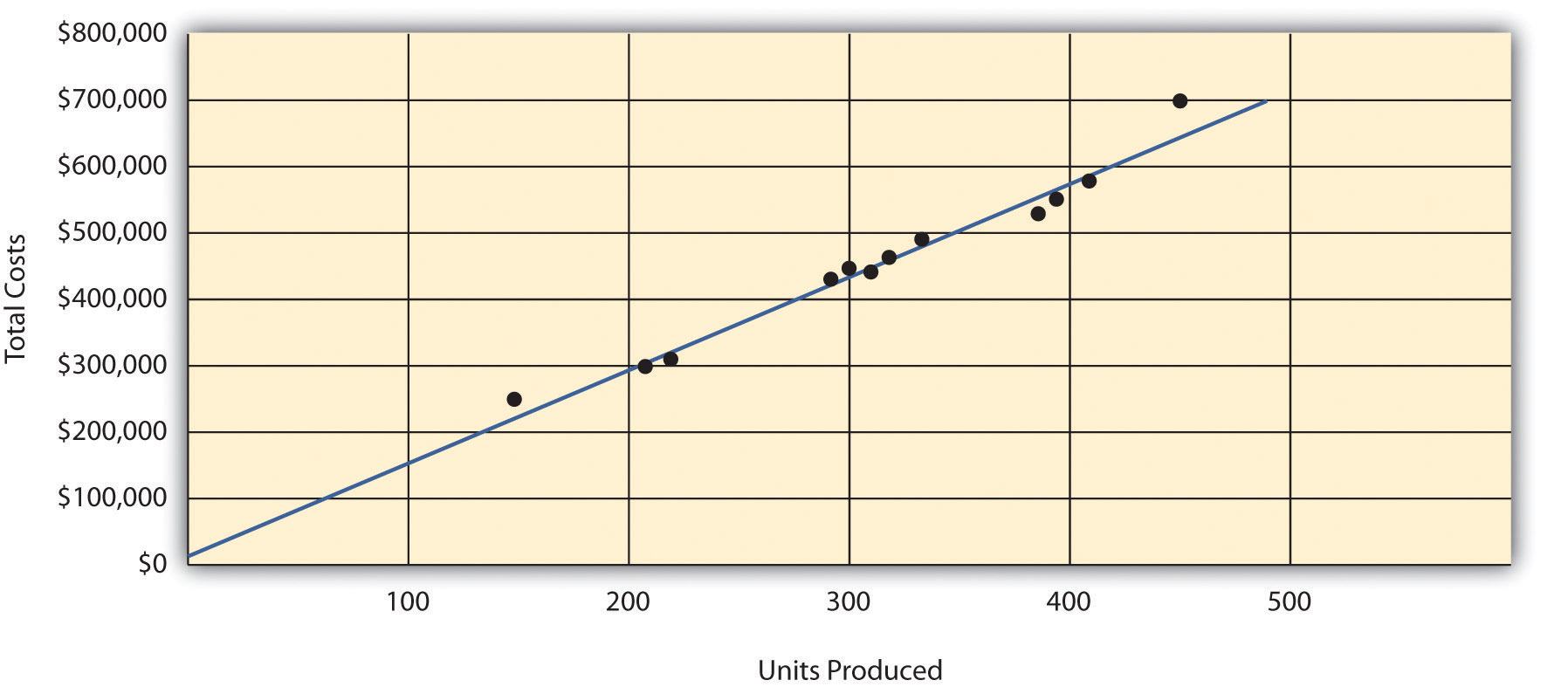
Once the data points are plotted as described in step 1, draw a line through the points touching one data point and extending to the y-axis. The goal here is to minimize the distance from the data points to the line (i.e., to make the line as close to the data points as possible). Figure 5.6 "Estimated Total Mixed Production Costs for Bikes Unlimited: Scattergraph Method" shows the line through the data points. Notice that the line hits the data point for July (3,500 units produced and $230,000 total cost).
Figure 5.6 Estimated Total Mixed Production Costs for Bikes Unlimited: Scattergraph Method
Step 3. Estimate the total fixed costs (f).
The total fixed costs are simply the point at which the line drawn in step 2 meets the y-axis. This is often called the y-intercept. Remember, the line meets the y-axis when the activity level (units produced in this example) is zero. Fixed costs remain the same in total regardless of level of production, and variable costs change in total with changes in levels of production. Since variable costs are zero when no units are produced, the costs reflected on the graph at the y-intercept must represent total fixed costs. The graph in Figure 5.6 "Estimated Total Mixed Production Costs for Bikes Unlimited: Scattergraph Method" indicates total fixed costs of approximately $45,000. (Note that the y-intercept will always be an approximation.)
Step 4. Calculate the variable cost per unit (v).
After completing step 3, the equation to describe the line is partially complete and stated as Y = $45,000 + vX. The goal of step 4 is to calculate a value for variable cost per unit (v). Simply use the data point the line intersects (July: 3,500 units produced and $230,000 total cost), and fill in the data to solve for v (variable cost per unit) as follows:
Thus variable cost per unit is $52.86.
Step 5. State the results in equation form Y = f + vX.
We know from step 3 that the total fixed costs are $45,000, and from step 4 that the variable cost per unit is $52.86. Thus the equation used to estimate total costs looks like this:
Y = $45,000 + $52.86XNow it is possible to estimate total production costs given a certain level of production (X). For example, if Bikes Unlimited expects to produce 6,000 units during August, total production costs are estimated to be $362,160:
Question: Remember that the key weakness of the high-low method discussed previously is that it considers only two data points in estimating fixed and variable costs. How does the scattergraph method mitigate this weakness?
Answer: The scattergraph method mitigates this weakness by considering all data points in estimating fixed and variable costs. The scattergraph method gives us an opportunity to review all data points in the data set when we plot these data points in a graph in step 1. If certain data points seem unusual (statistics books often call these points outliers), we can exclude them from the data set when drawing the best-fitting line. In fact, many organizations use a scattergraph to identify outliers and then use regression analysis to estimate the cost equation Y = f + vX. We discuss regression analysis in the next section.
Although the scattergraph method tends to yield more accurate results than the high-low method, the final cost equation is still based on estimates. The line is drawn using our best judgment and a bit of guesswork, and the resulting y-intercept (fixed cost estimate) is based on this line. This approach is not an exact science! However, the next approach to estimating fixed and variable costs—regression analysis—uses mathematical equations to find the best-fitting line.
Alta Production, Inc., reported the following production costs for the 12 months January through December. (These are the same data presented in Note 5.17 "Review Problem 5.3".)
| Reporting Period (Month) | Total Production Costs | Level of Activity (Units Produced) |
| January | $460,000 | 300 |
| February | 300,000 | 220 |
| March | 480,000 | 330 |
| April | 550,000 | 390 |
| May | 570,000 | 410 |
| June | 310,000 | 240 |
| July | 440,000 | 290 |
| August | 455,000 | 320 |
| September | 530,000 | 380 |
| October | 250,000 | 150 |
| November | 700,000 | 450 |
| December | 490,000 | 350 |
Solution to Review Problem 5.4
The five steps are as follows:
Step 1. Plot the data points for each period on a graph.
Step 2. Visually fit a line to the data points, and be sure the line touches one data point.
Step 3. Estimate the total fixed costs (f).
The y-intercept represents total fixed costs. This is where the line meets the y-axis. Total fixed costs in the graph appear to be approximately $5,000. You will likely get a different answer because the answer depends on the line that you visually fit to the data points. Remember you must draw the line through one data point. The line intersects the data point for March ($480,000 production costs; 330 units produced). This will be used in step 4.
Step 4. Calculate the variable cost per unit (v).
After completing step 3, the equation to describe the line is partially complete and stated as Y = $5,000 + vX. The goal of this step is to calculate a value for variable cost per unit (v). Use the data point the line intersects (for March, 330 units produced and $480,000 total costs), and fill in the data to solve for v (variable cost per unit):
Step 5. State the results in equation form Y = f + vX.
We know from step 3 that the total fixed costs are $5,000, and from step 4 that variable cost per unit is $1,439.39. Thus the equation used to estimate total production costs is stated as:
It is evident from this information that this company has very little in fixed costs and relatively high variable costs. This is indicative of a company that uses a high level of labor and materials (both variable costs) and a low level of machinery (typically a fixed cost through depreciation or lease costs).
Using the equation, simply substitute 400 units for X, as follows:
Thus total production costs are expected to be $580,756 for next month.
Question: Regression analysis is similar to the scattergraph approach in that both fit a straight line to a set of data points to estimate fixed and variable costs. How does regression analysis differ from the scattergraph method for estimating costs?
Answer: Regression analysisA method of cost analysis that uses a series of mathematical equations to estimate fixed and variable costs; typically done using computer software. uses a series of mathematical equations to find the best possible fit of the line to the data points and thus tends to provide more accurate results than the scattergraph approach. Rather than running these computations by hand, most companies use computer software, such as Excel, to perform regression analysis. Using the data for Bikes Unlimited shown back in Table 5.4 "Monthly Production Costs for Bikes Unlimited", regression analysis in Excel provides the following output. (This is a small excerpt of the output; see the appendix to this chapter for an explanation of how to use Excel to perform regression analysis.)
| Coefficients | |
| y-intercept | 43,276 |
| x variable | 53.42 |
Thus the equation used to estimate total production costs for Bikes Unlimited looks like this:
Y = $43,276 + $53.42XNow it is possible to estimate total production costs given a certain level of production (X). For example, if Bikes Unlimited expects to produce 6,000 units during August, total production costs are estimated to be $363,796:
Regression analysis tends to yield the most accurate estimate of fixed and variable costs, assuming there are no unusual data points in the data set. It is important to review the data set first—perhaps in the form of a scattergraph—to confirm that no outliers exist.
Alta Production, Inc., reported the following production costs for the 12 months January through December. (These are the same data that appear in Note 5.17 "Review Problem 5.3" and Note 5.19 "Review Problem 5.4".)
| Reporting Period (Month) | Total Production Cost | Level of Activity (Units Produced) |
| January | $460,000 | 300 |
| February | 300,000 | 220 |
| March | 480,000 | 330 |
| April | 550,000 | 390 |
| May | 570,000 | 410 |
| June | 310,000 | 240 |
| July | 440,000 | 290 |
| August | 455,000 | 320 |
| September | 530,000 | 380 |
| October | 250,000 | 150 |
| November | 700,000 | 450 |
| December | 490,000 | 350 |
Regression analysis performed using Excel resulted in the following output:
| Coefficients | |
| y-intercept | 703 |
| x variable | 1,442.97 |
Solution to Review Problem 5.5
The cost equation using the data from regression analysis is:
Using the equation, simply substitute 400 units for X, as follows:
Thus total production costs are expected to be $577,891 for next month.
Question: You are now able to create the cost equation Y = f + vX to estimate costs using four approaches. What does the cost equation look like for each approach at Bikes Unlimited?
Answer: The results of these four approaches for Bikes Unlimited are summarized as follows:
Question: We have seen that different methods yield different results, so which method should be used?
Answer: Regression analysis tends to be most accurate because it provides a cost equation that best fits the line to the data points. However, the goal of most companies is to get close—the results do not need to be perfect. Some could reasonably argue that the account analysis approach is best because it relies on the knowledge of those who are familiar with the costs involved.
At Bikes Unlimited, Eric (CFO) and Susan (cost accountant) met several days later. After consulting with her staff, Susan agreed that regression analysis was the best approach to use in estimating total production costs (keep in mind nothing has been done yet with selling and administrative expenses). Account analysis was ruled out because no one on the accounting staff had been with the company long enough to review the accounts and determine which costs were variable, fixed, or mixed. The high-low method was ruled out because it only uses two data points and Eric would prefer a more accurate estimate. Susan did request that her staff prepare a scattergraph and review it for any unusual data points before performing regression analysis. Based on the scattergraph prepared, all agreed that the data was relatively uniform and no outlying data points were identified.
| Susan: | My staff has been working hard to determine what will happen to profit if sales volume increases. So far, we’ve been able to identify cost behavior patterns for production costs, and we’re currently working on the cost behavior patterns for selling and administrative expenses. |
| Eric: | What do you have for production costs? |
| Susan: | The portion of production costs that are fixed—that won’t change with changes in production and sales—totals $43,276. The portion of production costs that are variable—that vary with changes in production and sales—totals $53.42 per unit. |
| Eric: | When do you expect to have further information for the selling and administrative costs? |
| Susan: | We should have those results by the end of the day tomorrow. At that point, I’ll put together an income statement projecting profit for August. |
| Eric: | Sounds good. Let’s meet when you have the information ready. |
Use the solutions you prepared for Note 5.15 "Review Problem 5.2", Note 5.17 "Review Problem 5.3", Note 5.19 "Review Problem 5.4", and Note 5.21 "Review Problem 5.5" to do the following:
Solution to Review Problem 5.6
The cost equations for each of the four methods used in Note 5.15 "Review Problem 5.2", Note 5.17 "Review Problem 5.3", Note 5.19 "Review Problem 5.4", and Note 5.21 "Review Problem 5.5" are shown here. Each of these cost equations was created using the same historical production cost data for Alta Production, Inc. The goal for you as a student is to understand how to develop a cost equation that will help in estimating costs for the future (based on past information).
Total production costs assuming 400 units will be produced are calculated for each method given. Note that the equations presented previously are used for these calculations.
Account analysis
High-low method
Scattergraph method
Regression analysis
The account analysis ($578,428), scattergraph method ($580,756), and regression analysis ($577,891) all yield similar estimated production costs. The high-low method varies significantly from the other three approaches, likely because only two data points are used to estimate unit variable cost and total fixed costs.


