Here are two recent headlines. The first discusses beer prices in England.
The average price of a pint of beer could hit £4 [about $8]…
Scottish & Newcastle today forecast “material price increases” next year. The brewer, which sells three of the top 10 beer brands in Europe including Kronenbourg and Foster’s, is also reviewing its supply chain in a bid to cut costs.
Industry experts say the cost of an average pint will rise by at least 15p, although some are now predicting rises of up to 60%.…
“It is a bleak time for everyone,” said Iain Lowe, research and information manager at Camra [The Campaign for Real Ale]. “These price rises have been predicted for a long time.”Teena Lyons, “The Price of a Pint Could Rise 60%,” Guardian Unlimited, November 20, 2007, accessed January 27, 2011, http://www.guardian.co.uk/business/2007/nov/20/fooddrinks.foodanddrink?gusrc=rss&feed=networkfront.
The second concerns sales of baseball merchandise in Detroit at the start of the 2010 season.
Opening Day is still a day away for Detroit’s baseball fans, but its impending arrival already is generating its share of Detroit Tiger retail hits.
Thousands of fans have flooded Comerica Park’s pro shop and other Metro Detroit sporting outlets in anticipation of Friday afternoon’s home game against the Cleveland Indians, snapping up Tigers jerseys, T-shirts and hats bearing the surnames Cabrera, Verlander and Damon, even Granderson—Tigers old and new.
…
Though it’s too soon to tell which Tigers will prove most popular at the checkout line, former players have been relegated to the discount bin.
“Retailers take a pretty aggressive stand,” Powell said. Most shops have marked down jerseys and T-shirts branded with ex-Tigers between 25 and 50 percent.
“Granderson and Polanco—we discount the price,” said Brian King, owner of Sports Authentics in Rochester Hills. “Unfortunately, you can’t take the names off the back.”“Tigers’ Merchandise off to Roaring Start,” The Detroit News, April 8, 2010, accessed January 27, 2011, http://www.detnews.com/article/20100408/BIZ/4080349/1129/Tigers-merchandise-off-to-roaring-start.
We could have picked thousands of other examples. If you search Google’s news aggregator on any day with a string such as “an increase in the price of” you will find dozens, perhaps hundreds, of recent news articles that contain this phrase. Our task in this chapter is to see where all these price changes come from and what they imply for other economic variables, such as the quantity of these goods traded.
To see how good you are at this, think about these two stories. Can you explain why the price of beer increased? Can you explain why “Granderson” T-shirts are being sold at discounted prices? What do you think happened to the quantity of beer sold as the price increased? What do you think happened to the quantity of T-shirts sold as the price decreased?
Understanding the sources and consequences of changing prices in the economy is one of the most important tasks of an economist. There is an almost endless list of such analyses in economics. In fact, most of the applications in this textbook ultimately come down to understanding, explaining, and predicting changes in prices. The question that motivates this chapter is so important that we have chosen it as the title:
Why do prices change?
All prices in the economy are ultimately chosen by someone. Sometimes they are chosen by marketing or pricing managers in big companies. Sometimes they are chosen by bidders in an auction. Sometimes they are agreed on by the buyer and the seller after bargaining.We discuss these choices in Chapter 5 "eBay and craigslist" and Chapter 6 "Where Do Prices Come From?". Yet we can often make good predictions about prices without looking closely at the individual decision making of buyers and sellers by summarizing their decisions with demand curves and supply curves. Building on the ideas of the individual demand curve and a firm’s supply curve for a good or service, we develop the ideas of supply and demand for an entire market.Individual demand and supply curves are introduced in Chapter 3 "Everyday Decisions" and Chapter 6 "Where Do Prices Come From?". In this chapter, we look at the trade that occurs between firms and households or among different firms in the economy. In the business world, these are called business-to-consumer (B2C) and business-to-business (B2B) trade, respectively. The market demand and supply curves that we derive allow us to predict what will happen to prices and quantities traded when there are changes that influence the market.Chapter 5 "eBay and craigslist" also looks at supply and demand in the context of trade between individuals.
An old joke says that you can ask an economist any question, and he will always give the same answer: supply and demand. Yet—strictly speaking—we are supposed to use the supply-and-demand framework only when we are talking about a competitive market—a market in which a homogeneous good is traded by a large number of buyers and sellers. In practice, economists and others use the framework all the time in settings where these assumptions do not hold. Perhaps surprisingly, this can be a completely reasonable thing to do, and we explain why.
Once we understand why prices change, we consider the implications of these price changes for the functioning of the economy. Prices convey information to both producers and consumers. When the price of a good or a service increases, it encourages consumers to consume less and producers to produce more. As we will see, this means that prices play a crucial role in allocating resources in the economy.
We finish this chapter by looking at three very significant markets in the economy: the labor market, the credit market, and the foreign exchange market. Understanding how these three markets work is necessary for a good understanding of both microeconomics and macroeconomics.
We begin the chapter with the individual demand curve—sometimes also called the household demand curve—that is based on an individual’s choice among different goods. (In this chapter, we use the terms individual and household interchangeably.) We show how to build the market demand curve from these individual demand curves. Then we do the same thing for supply, showing how to build a market supply curve from the supply curves of individual firms. Finally, we put them together to obtain the market equilibrium.
Figure 7.1 "The Demand Curve of an Individual Household" is an example of a household’s demand for chocolate bars each month. Taking the price of a chocolate bar as given, as well as its income and all other prices, the household decides how many chocolate bars to buy. Its choice is represented as a point on the household’s demand curve. For example, at $5, the household wishes to consume five chocolate bars each month. The remainder of the household income—which is its total income minus the $25 it spends on chocolate—is spent on other goods and services. If the price decreases to $3, the household buys eight bars every month. In other words, the quantity demanded by the household increases. Equally, if the price of a chocolate bar increases, the quantity demanded decreases. This is the law of demand in operation.
One way to summarize this behavior is to say that the household compares its marginal valuation from one more chocolate bar to price. The marginal valuation is a measure of how much the household would like one more chocolate bar. The household will keep buying chocolate bars up to the point where
marginal valuation = price.Toolkit: Section 17.1 "Individual Demand"
You can review the foundations of individual demand and the idea of marginal valuation in the toolkit.
Figure 7.1 The Demand Curve of an Individual Household
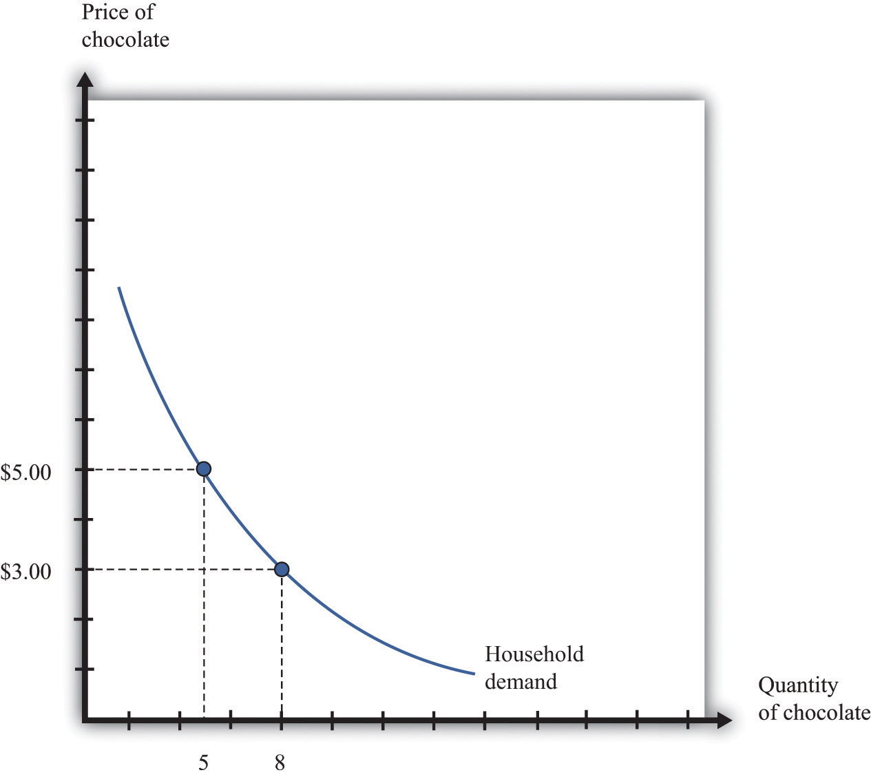
The household demand curve shows the quantity of chocolate bars demanded by an individual household at each price. It has a negative slope: higher prices lead people to consume fewer chocolate bars.
Table 7.1 Individual and Market Demand
| Price ($) | Household 1 Demand | Household 2 Demand | Market Demand |
|---|---|---|---|
| 1 | 17 | 10 | 27 |
| 3 | 8 | 3 | 11 |
| 5 | 5 | 2 | 7 |
| 7 | 4 | 1.5 | 5.5 |
In most markets, many households purchase the good or the service traded. We need to add together all the demand curves of the individual households to obtain the market demand curve. To see how this works, look at Table 7.1 "Individual and Market Demand" and Figure 7.2 "Market Demand". Suppose that there are two households. Part (a) of Figure 7.2 "Market Demand" shows their individual demand curves. Household 1 has the demand curve from Figure 7.1 "The Demand Curve of an Individual Household". Household 2 demands fewer chocolate bars at every price. For example, at $5, household 2 buys 2 bars per month; at $3, it buys 3 bars per month. To get the market demand, we simply add together the demands of the two households at each price. For example, when the price is $5, the market demand is 7 chocolate bars (5 demanded by household 1 and 2 demanded by household 2). When the price is $3, the market demand is 11 chocolate bars (8 demanded by household 1 and 3 demanded by household 2). When we carry out the same calculation at every price, we get the market demand curve shown in part (b) of Figure 7.2 "Market Demand".
Toolkit: Section 17.9 "Supply and Demand"
You can review the market demand curve in the toolkit.
Figure 7.2 Market Demand
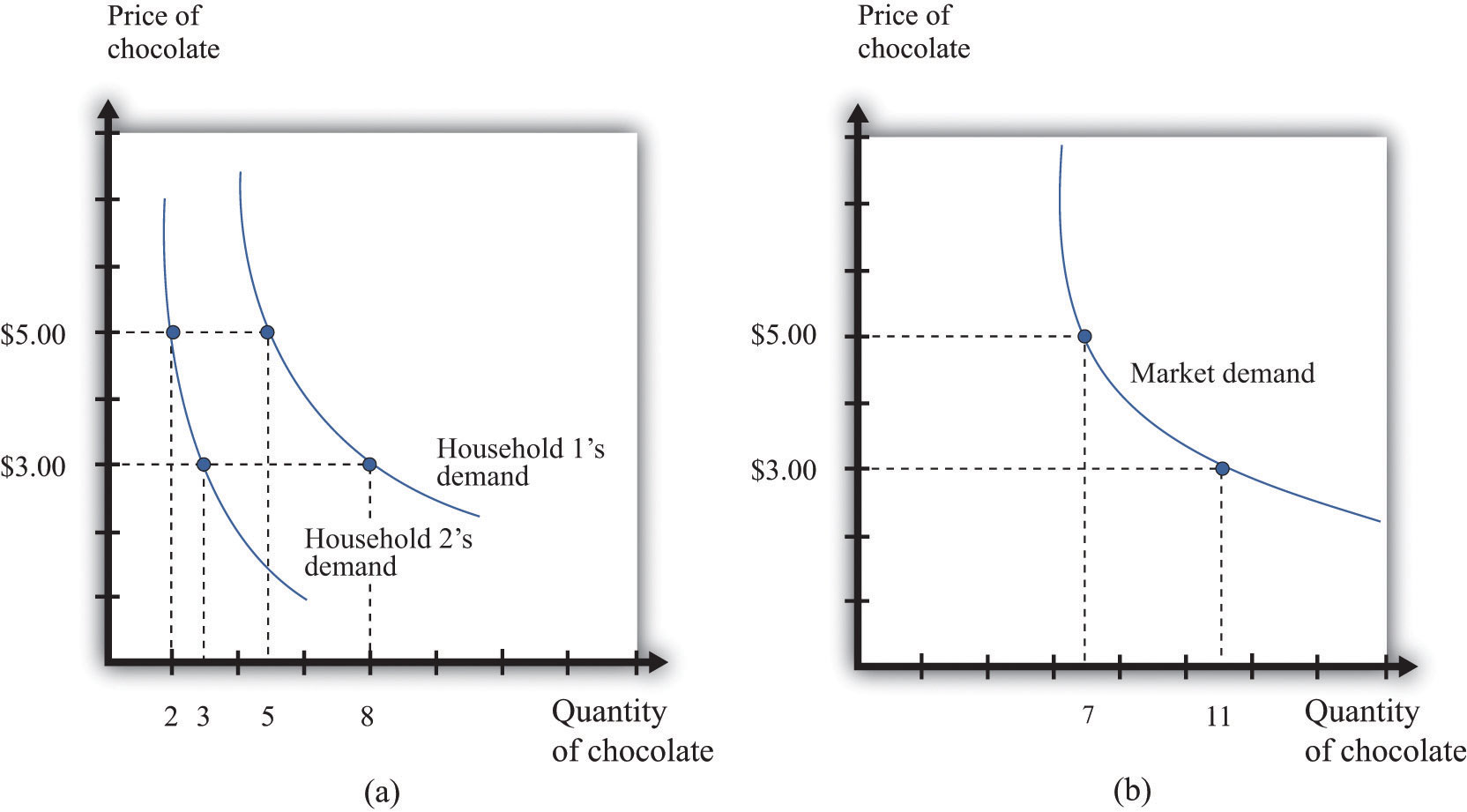
Market demand is obtained by adding together the individual demands of all the households in the economy.
Because the individual demand curves are downward sloping, the market demand curve is also downward sloping: the law of demand carries across to the market demand curve. As the price decreases, each household chooses to buy more of the product. Thus the quantity demanded increases as the price decreases. Although we used two households in this example, the same idea applies if there are 200 households or 20,000 households. In principle, we could add together the quantities demanded at each price and arrive at a market demand curve.
There is a second reason why demand curves slope down when we combine individual demand curves into a market demand curve. Think about the situation where each household has a unit demand curve: that is, each individual buys at most one unit of the product. As the price decreases, the number of individuals electing to buy increases, so the market demand curve slopes down.See Chapter 3 "Everyday Decisions" and Chapter 5 "eBay and craigslist" for discussions of unit demand. In general, both mechanisms come into play.
When the price decreases, there are more buyers, and each buyer buys more.
In a competitive marketA market that satisfies two conditions: (1) there are many buyers and sellers, and (2) the goods the sellers produce are perfect substitutes., a single firm is only one of the many sellers producing and selling exactly the same product. The demand curve facing a firm exhibits perfectly elastic demand, which means that it sets its price equal to the price prevailing in the market, and it chooses its output such that this price equals its marginal costThe extra cost of producing an additional unit of output, which is equal to the change in cost divided by the change in quantity. of production.At the end of Chapter 6 "Where Do Prices Come From?", we derive the supply curve of a firm in a competitive market. If it were to try to set a higher price, it could not sell any output at all. If it were to set a lower price, it would be throwing away profits. Thus, for a competitive firm, the quantity produced satisfies this condition:
price = marginal cost.Toolkit: Section 17.2 "Elasticity"
For more information on elasticity, see the toolkit.
We typically expect that marginal cost will increase as a firm produces more output. Marginal cost is the cost of producing one extra unit of output. The cost of producing an additional unit of output generally increases as firms produce a larger and larger quantity. In part, this is because firms start to hit constraints in their capacities to produce more product. For example, a factory might be able to produce more output only by running extra shifts at night, which require paying higher wages.
If marginal cost is increasing, then we know the following:
Indeed, the supply curve of an individual firm is the same as its marginal cost curve.
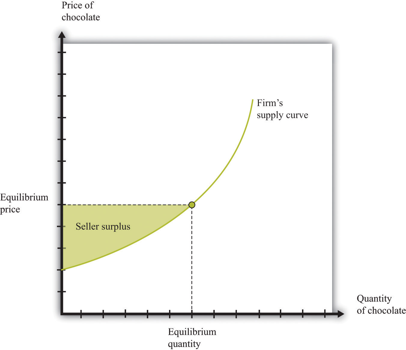
Figure 7.3 "The Supply Curve of an Individual Firm" illustrates the supply curve for a firm. A firm supplies seven chocolate bars at $3 and eight chocolate bars at $5. From this we can deduce that the marginal cost of producing the seventh chocolate bar is $3. Similarly, the marginal cost of producing the eighth chocolate bar is $5.
Figure 7.3 The Supply Curve of an Individual Firm
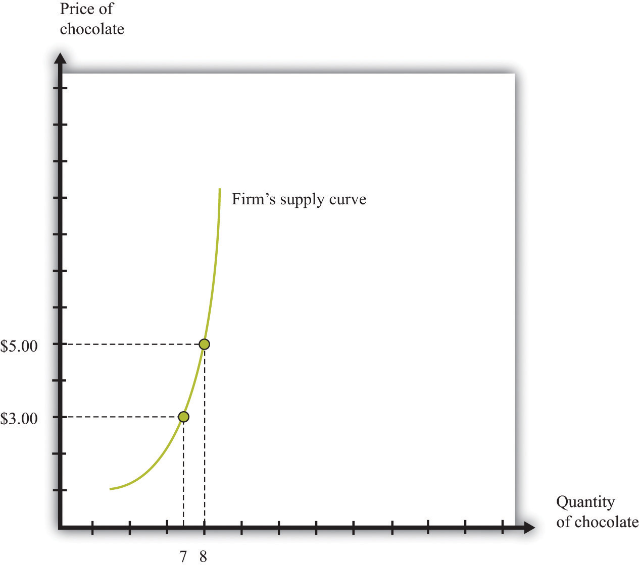
A firm’s supply curve, which is the same as its marginal cost curve, shows the quantity of chocolate bars it is willing to supply at each price.
Just as the market demand curve tells us the total amount demanded at each price, the market supply curve tells us the total amount supplied at each price. It is obtained analogously to the market demand curve: at each price we add together the quantity supplied by each firm to obtain the total quantity supplied at that price. If we perform this calculation for every price, then we get the market supply curve. Figure 7.4 "Market Supply" shows an example with two firms. At $3, firm 1 produces 7 bars, and firm 2 produces 3 bars. Thus the total supply at this price is 10 chocolate bars. At $5, firm 1 produces 8 bars, and firm 2 produces 5 bars. Thus the total supply at this price is 13 chocolate bars.
The market supply curve is increasing in price. As price increases, each firm in the market finds it profitable to increase output to ensure that price equals marginal cost. Moreover, as price increases, firms who choose not to produce and sell a product may be induced to enter into the market.A similar idea is in Chapter 5 "eBay and craigslist", where we show how to add together unit supply curves to obtain a market supply curve.
Figure 7.4 Market Supply
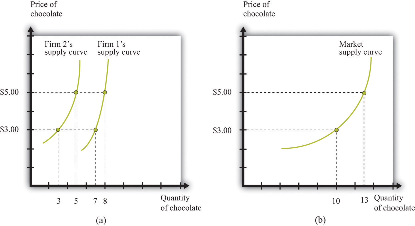
Market supply is obtained by adding together the individual supplies of all the firms in the economy.
In general, both mechanisms come into play. The market supply curve slopes up for two reasons:
When the price increases, there are more firms in the market, and each firm produces more.
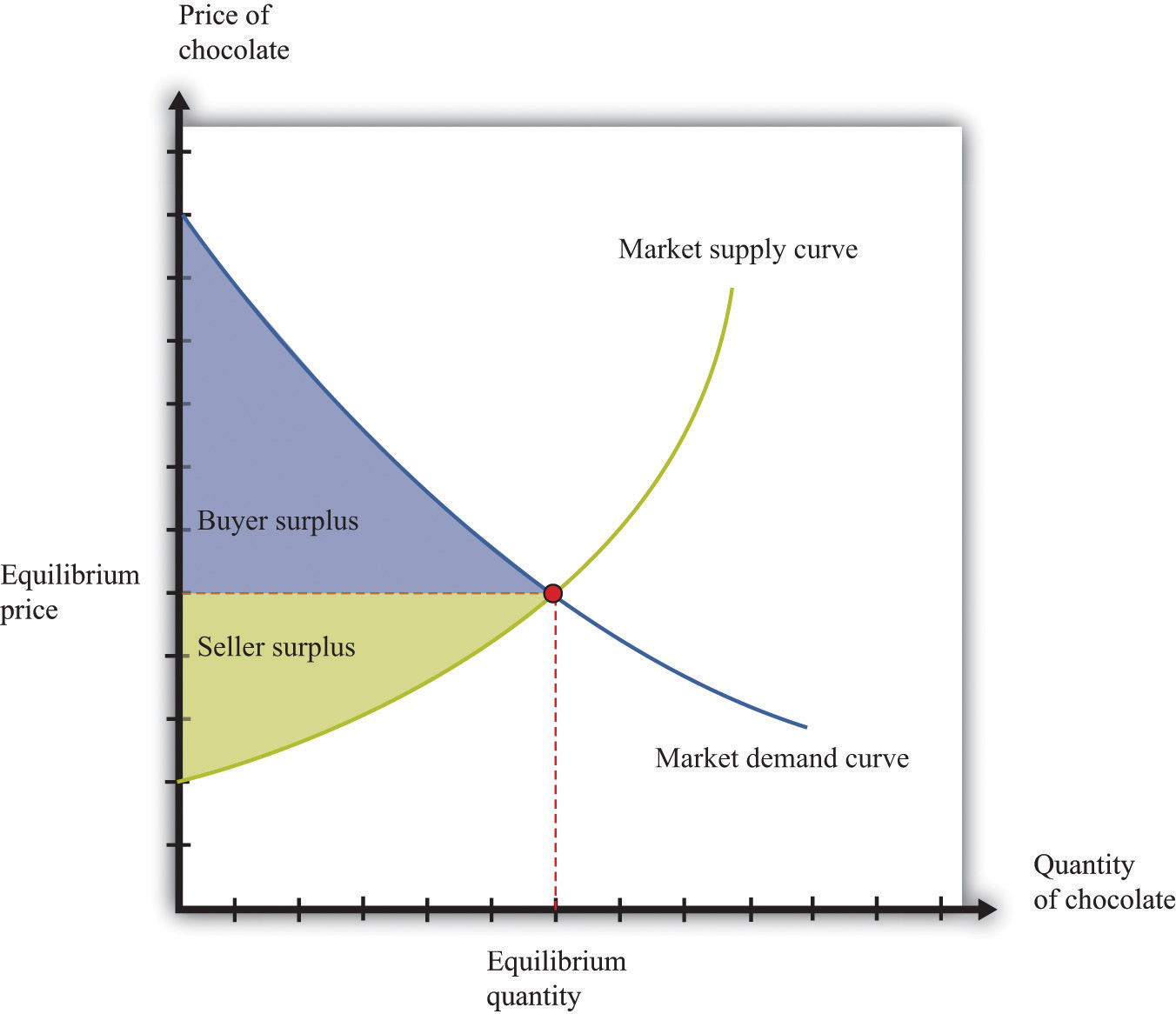
In a perfectly competitive market, we combine the market demand and supply curves to obtain the supply-and-demand framework shown in Figure 7.5 "Market Equilibrium". The point where the curves cross is the market equilibrium.The definition of equilibrium is also presented in Chapter 5 "eBay and craigslist". At this point, there is a perfect match between the amount that buyers want to buy and the amount that sellers want to sell. The term equilibrium refers to the balancing of the forces of supply and demand in the market. At the equilibrium price, the suppliers of a good can sell as much as they wish, and demanders of a good can buy as much of the good as they wish. There are no disappointed buyers or sellers.
Toolkit: Section 17.9 "Supply and Demand"
You can review the definition and meaning of equilibrium in the supply-and-demand framework in the toolkit.
Figure 7.5 Market Equilibrium
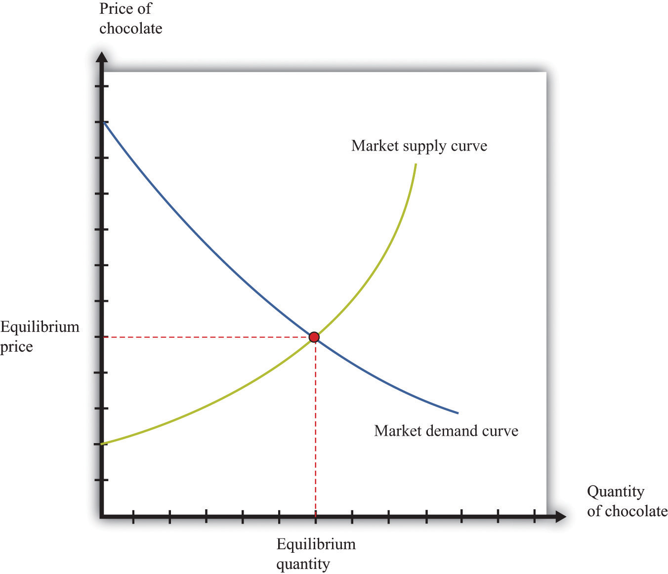
In a competitive market, the equilibrium price and the equilibrium quantity are determined by the intersection of the supply and demand curves.
Because the demand curve has a negative slope and the supply curve has a positive slope, supply and demand will cross once. Both the equilibrium price and the equilibrium quantity will be positive. (More precisely, this is true as long as the vertical intercept of the demand curve is larger than the vertical intercept of the supply curve. If this is not the case, then the most that any buyer is willing to pay is less than the least any seller is willing to accept and there is no trade in the market.)
Table 7.2 Market Equilibrium: An Example
| Price ($) | Market Supply | Market Demand |
|---|---|---|
| 1 | 5 | 95 |
| 5 | 25 | 75 |
| 10 | 50 | 50 |
| 20 | 100 | 0 |
Table 7.2 "Market Equilibrium: An Example" shows an example of market equilibrium with market supply and market demand at four different prices. The equilibrium occurs at $10 and a quantity of 50 units. The table is based on the following equations:
market demand = 100 − 5 × priceand
market supply = 5 × price.Equations such as these and diagrams such as Figure 7.5 "Market Equilibrium" are useful to economists who want to understand how the market works. Keep in mind, though, that firms and households in the market do not need any of this information. This is one of the beauties of the market. An individual firm or household needs to know only the price that is prevailing in the market.
Economists typically believe that a perfectly competitive market is likely to reach equilibrium for several reasons.
Economists are often asked to make predictions about the effects of events on economic outcomes. They do so by using the supply-and-demand framework. To use this framework, we must first distinguish between those things that we take as given (exogenousSomething that comes from outside a model and is not explained in our analysis. variables) and those that we seek to explain (endogenousSomething that is explained within our analysis. variables).
Toolkit: Section 17.16 "Comparative Statics"
An exogenous variable is something that comes from outside a model and is not explained in our analysis. An endogenous variable is one that is explained within our analysis. When using the supply-and-demand framework, price and quantity are endogenous variables; everything else is exogenous.
Figure 7.6 A Shift in the Supply Curve of an Individual Firm
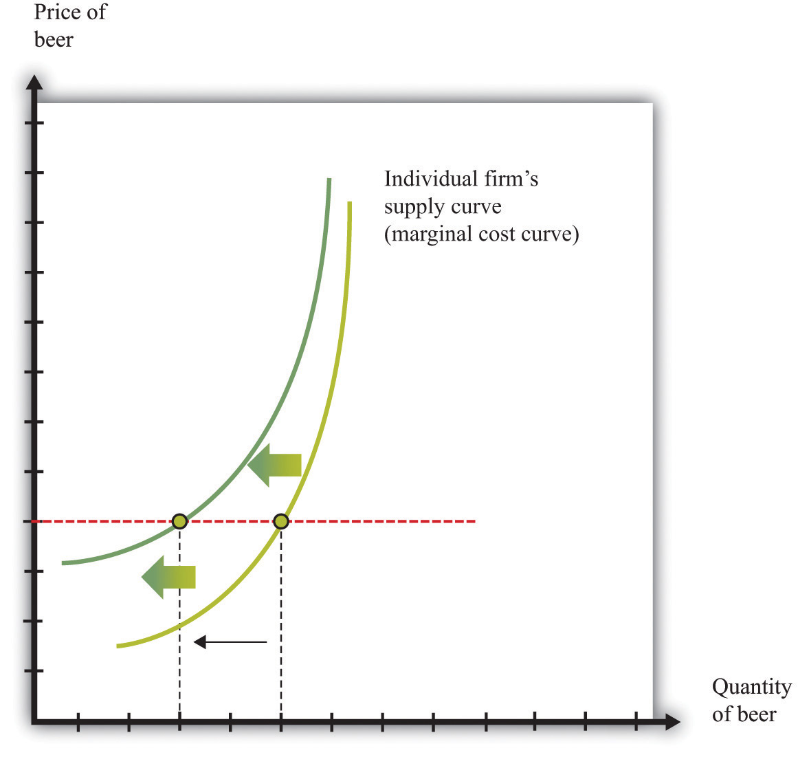
An increase in marginal cost leads a firm to produce less output at any given price. This means that a firm’s supply curve shifts upward and to the left.
When we quoted the British newspaper article about beer prices in the chapter introduction, we omitted some sentences. The first sentence reads, in full: “The average price of a pint of beer could hit £4 [pounds sterling] after poor weather forced up the price of hops.” A few sentences later the article states: “Hop farmers have not seen any price rises for years, but the appalling summer has finally forced the prices up.” According to the article, the price of beer is increasing because the price of hops has increased.
This makes intuitive sense, but it is worth understanding the exact chain of reasoning here. Hops are a key ingredient in the production of beer. An increase in the price of hops means an increase in the cost of producing beer. More precisely, the marginal cost of producing beer increases. The typical beer producer decides how much to produce by observing this decision rule:
price = marginal cost.If marginal cost increases, then, at the existing price, the producer will find that price is now less than marginal cost. To bring price back in line with marginal cost, the producer will have to produce a smaller quantity. In fact, at any given price, an increase in marginal cost leads to a reduction in output (Figure 7.6 "A Shift in the Supply Curve of an Individual Firm"). The supply curve of an individual firm shifts to the left.
The increase in the price of hops affects all firms in the market. Each firm sees an increase in its marginal cost of production, so each firm produces less output at a given price: the shift in supply shown in Figure 7.6 "A Shift in the Supply Curve of an Individual Firm" applies to all firms in the market. Figure 7.7 "A Shift in Market Supply" shows the outcome in the market. Because all the individual supply curves shift to the left, the market supply curve likewise shifts to the left. At any given price, firms supply less beer to the market. From the figure, we see that the higher price of hops leads to an increase in the price of beer and a reduction in the quantity of beer produced and sold.
Figure 7.7 A Shift in Market Supply
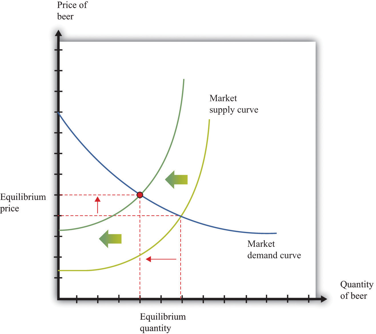
An increase in the price of hops causes all beer producers to produce less at any given price. This means that the market supply curve shifts to the left. The consequence is an increase in the equilibrium price and a decrease in the equilibrium quantity.
For the individual producer, what does this mean? The producer sees an increase in marginal cost. In the new equilibrium, the producer also obtains a higher price. However, the increase in price is not as big as the increase in marginal cost. Because the producer sets price equal to marginal cost, each individual brewer still produces less. We show this in Figure 7.8 "The New Equilibrium from the Perspective of an Individual Firm".
Figure 7.8 The New Equilibrium from the Perspective of an Individual Firm
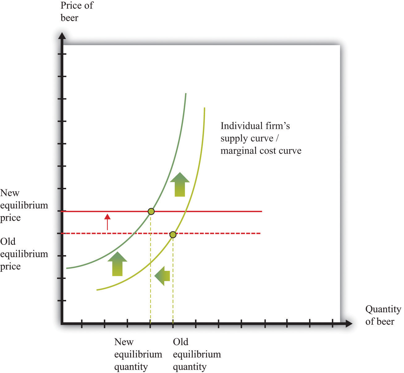
Following the increase in the price of hops, the equilibrium price of beer increases. An individual firm ends up with higher marginal cost but also receives a higher price for beer. Because the increase in price is smaller than the increase in marginal cost, beer production still decreases.
The approach that we used here is an illustration of a general technique used by economists to explain changes in prices and quantities and to make predictions about what will happen to market prices.
Toolkit: Section 17.16 "Comparative Statics"
Comparative statics is a technique that allows us to describe how market equilibrium prices and quantities depend on exogenous events. As such, much of economics consists of exercises in comparative statics. In a comparative statics exercise, you must do the following:
The most difficult part of a comparative staticsA technique that allows us to describe how market equilibrium prices and quantities depend on exogenous events. exercise is to determine, from the description of the economic problem, which curve to shift—supply or demand. Once you determine which curve is shifting, then it is only a matter of using the supply-and-demand framework to find the new equilibrium. The final step is to compare the new equilibrium point (the new crossing of supply and demand) with the original point. With this comparison, you can predict what will happen to equilibrium prices and quantities when something exogenous changes.
Let us try this technique again. Recall the second story from the chapter introduction about Detroit Tiger merchandise. In that story, we learned that “most shops have marked down jerseys and T-shirts branded with ex-Tigers between 25 and 50 percent.” Figure 7.9 "Shifts in Household Demand" shows the demand of a typical Detroit household’s demand for Granderson shirts. Now that Granderson has left the Tigers for the New York Yankees, the household’s marginal valuation for these shirts is lower. At any given price, a household wants to purchase fewer shirts, so the household’s demand curve shifts to the left.
Figure 7.9 Shifts in Household Demand
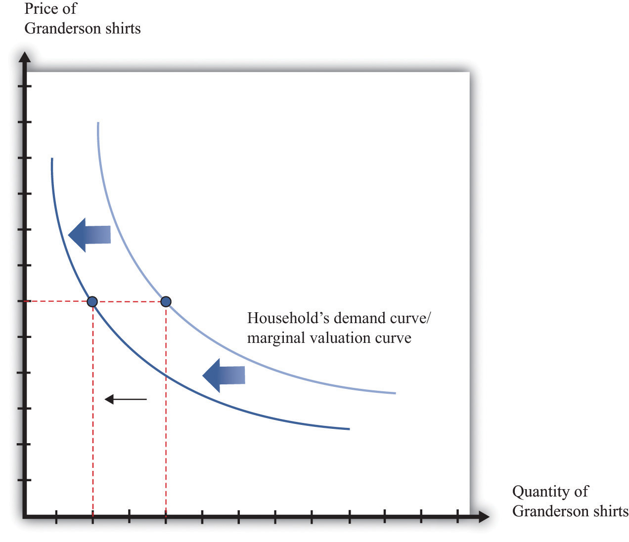
A decrease in the marginal valuation of Granderson T-shirts leads a household to demand a smaller quantity at any given price. This means that a household’s demand curve shifts to the left.
We would expect that this shift in demand would apply to most households that contain Detroit Tigers fans. If we now add all the demand curves together, we get the market demand curve. The market demand curve shifts to the left (Figure 7.10 "Shifts in Market Demand"). The end result is that we expect to see a decrease in the price of T-shirts—that is, the retailers put them in the discount bins—and also a decrease in demand.
Figure 7.10 Shifts in Market Demand
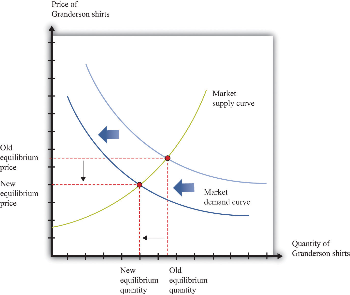
The decrease in demand causes both the equilibrium price and the equilibrium quantity of T-shirts to decrease.
Comparing our beer and T-shirt examples, we see that the quantity demanded decreased in both examples. In the first case, price increased; in the second case, price decreased. We can understand the difference by using the supply-and-demand framework. In the Detroit Tigers example, there is a decrease in the price of shirts and in the quantity sold. This might seem like a violation of the law of demand, which tells us that when price decreases, the quantity demanded increases. The explanation comes directly from Figure 7.10 "Shifts in Market Demand".
Curtis Granderson’s move leads to a shift in the demand curve and a movement along the supply curve. The law of demand, by contrast, applies to the movement along a demand curve.
Understanding the distinction between moving along a curve (either supply or demand) and shifting a curve is the hardest part about learning to use the supply-and-demand framework. Journalists and others frequently are confused about this—and no wonder. It requires practice to learn how to use supply and demand properly.
Let’s look at another example. An article in the British newspaper the Guardian reported about sales of beef when the news came out that eating beef might carry a risk of bovine spongiform encephalopathy (BSE), better known as mad cow disease. On November 1, 2000, the newspaper wrote, “Beef sales did drop after the link between BSE and deaths in humans was circumstantially established in 1996, but they have recovered as prices have fallen.”“First Beef—Now Lamb to the Slaughter?” Analysis, Guardian, November 1, 2000, accessed February 4, 2011, http://www.guardian.co.uk/uk/2000/nov/01/bse?INTCMP=SRCH.
The exogenous event here is the medical news about beef and mad cow disease. Presumably, this primarily affects the demand for beef: consumers decide to eat less beef and more of other products—such as chicken and pork. The demand curve for beef shifts to the left. As we saw in the T-shirt example, a leftward shift of the demand curve has two consequences: price decreases, and the quantity demanded and supplied also decreases. Thus the conclusion that the news should lead to a decrease in beef sales is perfectly consistent with our supply-and-demand analysis, as well as with common sense.
But what about the second part of the sentence? The article claims that beef sales “have recovered as prices have fallen.” This is not consistent with our supply-and-demand analysis. The decrease in prices is intimately connected with the decrease in quantity: both were caused by the health news. They are two sides of the same coin, so it does not make sense to use the decrease in prices to explain a recovery in beef sales.
In fact, you should be able to convince yourself that an increase in beef sales together with a decrease in prices (as asserted by the article) would require a rightward shift of the supply curve. (Draw a diagram to make sure you understand this.) It seems unlikely that health concerns about beef led cattle farmers to increase their production of beef. It is hard to escape the conclusion that the journalist became confused about shifts in the demand curve and movements along the curve.
Comparative statics allows us to make qualitative predictions about prices and quantities. Given an exogenous shock in a market, we can determine whether (1) the price is likely to increase or decrease and (2) the quantity bought and sold is likely to increase or decrease. Often, though, we would like to be able to do more. We would like to be able to make some predictions about the magnitudes of the changes.
Figuring out what will happen to equilibrium prices and quantities requires economists to know the shapes of supply and demand. When the supply curve shifts, we need to know about the slope of the demand curve to predict the impact on price and quantity. When the demand curve shifts, we need to know about the slope of the supply curve to predict the impact on price and quantity. More precisely, we need measures of the elasticity of demand and of supply.
How do economists learn about these elasticities? The answer, perhaps surprisingly, is through the logic of comparative statics. For example, suppose the supply curve does not move, but the demand curve shifts around a lot. As the demand curve shifts, we observe different combinations of prices and quantities. Part (a) of Figure 7.11 "Finding the Elasticities of the Supply and Demand Curves" shows this in a supply-and-demand diagram. The different points that we observe are points on the supply curve. If the demand curve shifts but the supply curve does not, we eventually gather data on the supply curve. We can use these data to come up with estimates of the price elasticity of supplyThe percentage change in the quantity supplied to the market divided by the percentage change in price..
Toolkit: Section 17.2 "Elasticity"
The price elasticity of supply equals the percentage change in the quantity supplied divided by the percentage change in price.
Figure 7.11 Finding the Elasticities of the Supply and Demand Curves
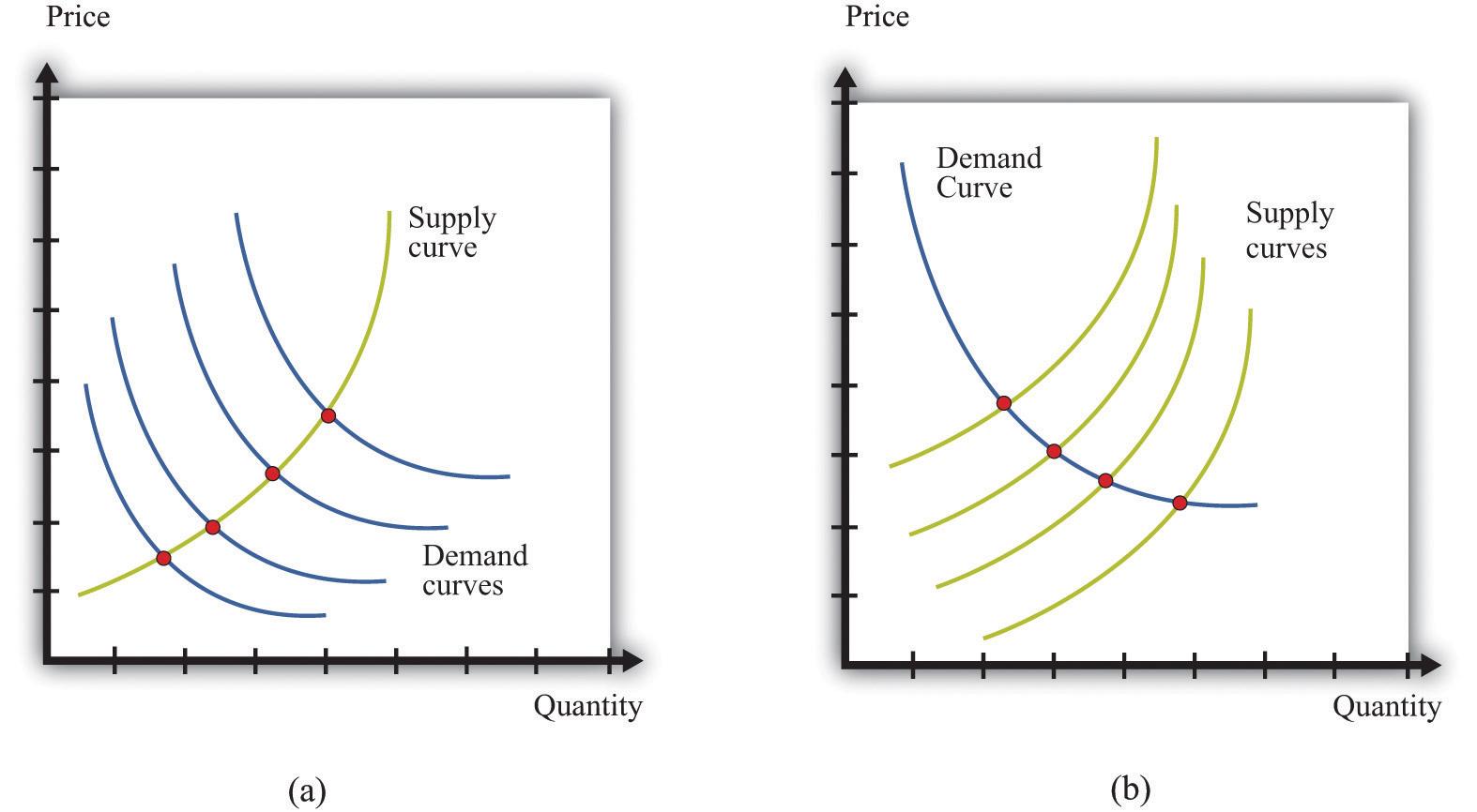
Economists estimate the elasticities of supply and demand curves by looking for situations in which one curve is relatively stable while the other one is moving. What we actually observe are the equilibrium points. Movements in the demand curve (a) mean that the equilibrium points trace out the supply curve; movements in the supply curve (b) allow us to observe the demand curve. In most real-life cases, both curves move, and economists use sophisticated statistical techniques to tease apart shifts in supply from shifts in demand.
Part (b) of Figure 7.11 "Finding the Elasticities of the Supply and Demand Curves" shows the opposite case, where demand is stable and the supply curve is shifting. In this case, the data that we observe are different points on the demand curve. We can use this information to estimate the price elasticity of demandThe percentage change in the quantity demanded in the market divided by the percentage change in price., which is the percentage change in the quantity demanded divided by the percentage change in price. It is important to note that we are speaking here about the elasticity of the market demand curve, not the elasticity of the demand curve facing an individual firm.
This sounds straightforward in theory, but it is difficult in practice. Economic data are messy. Typically, both the demand curve and the supply curve are shifting simultaneously. If economists had access to controlled environments, perhaps like a biochemist does, we could “shift the demand curve” and see what happens in the laboratory. Occasionally, we get lucky. Sometimes we can isolate a particular event that we know is likely to shift only one of the curves. This is sometimes called a natural experimentAn exogenous change that can be associated with a shift in either the demand curve only or the supply curve only.. Most of the time, however, we are not so lucky. Economists and statisticians have come up with sophisticated statistical techniques to disentangle shifts in demand and supply in these circumstances.Chapter 6 "Where Do Prices Come From?" discusses how a firm can use a similar technique to learn about the demand curve that it faces. Chapter 10 "Raising the Wage Floor" discusses the difficulties of measuring the demand curve for labor.
Think back to our story of increasing beer prices. In Figure 7.6 "A Shift in the Supply Curve of an Individual Firm", we saw that an increase in the marginal cost of beer production led to an increase in the price and a decrease in the quantity supplied. In that explanation, we focused on what was happening to supply. But as the supply curve shifted, we moved along the demand curve to a new equilibrium. What was happening to the quantity demanded as the quantity supplied decreased? The answer is that as firms started decreasing their supply, the price in the market began to increase. Consumers of beer, confronted by these higher prices, bought less beer. Perhaps they switched to wine or spirits instead. The higher prices induced the quantity demanded to decrease in line with the decline in supply.
Something remarkable is happening in this story, however. Bad weather has affected the hops harvest, making beer more expensive to produce, relative to other goods and services. Because it is more expensive to make beer, it makes sense—from the point of view of society as a whole—to shift resources away from the production of beer and toward the production of other goods. And it makes sense—from the point of view of society as a whole—for people to consume less of the expensive-to-produce beer and more of other goods and services. If we imagine an all-knowing, all-powerful central planner, whose job is to allocate resources in the economy, we would expect this person to respond to the decrease in the hops harvest by ordering the production and consumption of less beer.
But this is exactly what happens in an economy, simply through the mechanism of supply and demand. The automatic adjustment of prices, resulting from shifts in supply and demand, brings about desirable shifts in production and consumption. Nobody orders producers to produce less or consumers to consume less. These outcomes result from the working of supply and demand.
Similarly, think about our T-shirt example. Consumers decide that they would like to consume fewer Granderson T-shirts. This change in their preferences shows up in the market as a shift in the demand curve, which causes the price of T-shirts to decrease. This decrease in the price encourages producers in the economy to adjust their behavior to fit the changed tastes of households. Firms stop producing Granderson shirts. Again, this is not because anyone has instructed them to do so. The changed tastes of households generate the price signal that induces firms to produce less.
So far, we have answered the question of the chapter by saying that prices change because of shifts in supply and/or demand. This answer is correct. But we could give a different answer from another perspective: prices change in order to provide signals to firms and households about what to produce and what to consume. In a market economy, households and firms decide what to consumer by considering the prices they face. Prices change in response to changes in costs and tastes, and these changes lead firms and households to adjust their decisions in line with the new economic reality.
It is fair to ask whether we should trust prices to play this role. Economics provides a very direct answer to this question: when markets are competitive, the price system delivers an efficient allocation of resources. In the following subsections, we develop the idea that markets deliver efficient outcomes by looking at a single market.
Consider the market for chocolate bars, as shown in Figure 7.5 "Market Equilibrium". At the market clearing price, suppliers and demanders of chocolate bars trade the equilibrium quantity of chocolate bars. Imagine first that each household purchases no more than a single chocolate bar at the equilibrium price. For example, if 200 chocolate bars are sold, then 200 separate households bought a chocolate bar. Not all these households are alike, however: some like chocolate bars more than others. Most of them would have, in fact, been willing to pay more than the equilibrium price for the chocolate bar. Their valuation of a chocolate bar is greater than the price.
Any household that would have been willing to pay more than the equilibrium price gets a good deal. For example, suppose the equilibrium price is $5, but a household would have been willing to pay $7. Then that household receives a buyer surplus of $2.See Chapter 5 "eBay and craigslist" for more discussion. This logic extends to the case where households consume more than one unit. The demand curve of a household indicates the maximum amount that a person would pay for each successive unit of a good. The demand curve shows the household’s marginal valuation of a good. The individual household’s demand curve slopes downward because the household is willing to pay less and less for each successive unit—the marginal unit—as the total quantity consumed increases.
In general, we know that a household purchases chocolate bars up to the point where
marginal valuation = price.The household receives no surplus on the very last bar that it purchases because the marginal valuation of that bar equals price. But it receives surplus on all the other bars because its marginal valuation exceeds price for those bars. Diminishing marginal valuation means that the household obtains surplus from all the chocolate bars except the very last one.
Table 7.3 "Calculating Buyer Surplus for an Individual Household" gives an example of a household facing a price of $5. The first column is the quantity, the second is the price, the third is the marginal valuation (the extra value from the last chocolate), the fourth column measures the marginal surplus, and the last column is the total surplus.
Table 7.3 Calculating Buyer Surplus for an Individual Household
| Quantity (Bars) | Price | Marginal Valuation | Surplus for Marginal Unit | Total Surplus |
|---|---|---|---|---|
| 1 | 5 | 10 | 5 | 5 |
| 2 | 5 | 8 | 3 | 8 |
| 3 | 5 | 5 | 0 | 8 |
| 4 | 5 | 3 | –2 | 6 |
The household is willing to buy three chocolate bars because the marginal value of the third bar is exactly equal to the price of $5. (In fact, the household would be equally happy buying either two or three bars. It makes no substantive difference to the discussion, but it is easier if we suppose that the household buys the last bar even though it is indifferent about making this purchase.) The household would not buy four bars because the marginal valuation of the last unit is less than the price, which means the surplus from a fourth chocolate bar would be negative.
The household obtains surplus from the first and second bars that it purchases. The household would have been willing to pay $10 for the first bar but only had to pay $5. It gets $5 of surplus from this first bar. The household would have been willing to pay $8 for the second bar but only had to pay $5. It gets $3 of surplus for this second bar. It gets no surplus from the third bar. So the total buyer surplus for this household is $5 + $3 = $8. Notice that by following the rule “buy until marginal valuation equals price,” the household maximizes its total surplus from the purchase of chocolate bars.
More generally, the buyer surplus for this household is measured by the area under its demand curve (Figure 7.12 "Buyer Surplus for an Individual Household"). For each unit, the vertical difference between the price actually paid for each unit and the price the household would have been willing to pay measures the surplus earned for that unit. If we add the surplus over all units, we get the area between the demand curve and the price.
Figure 7.12 Buyer Surplus for an Individual Household
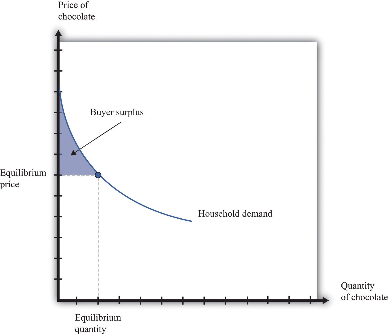
The buyer surplus is equal to the area between the demand curve and the price.
Sellers as well as buyers obtain surplus from trade. Suppose you won a used bicycle that you value at $20. If you can sell that bicycle for $30, you receive a seller surplus of $10—the difference between the price and your valuation of the good. It is worth your while to sell as long as the price is greater than your valuation. When a firm is producing a good for sale, the situation is analogous. If a firm can produce one more unit of a good at a marginal cost of $20, then the firm’s valuation of the good is effectively equal to $20. If the firm can sell that unit for $30, it will receive a surplus of $10. The seller surplus earned by a firm for an individual unit is the difference between price and the marginal cost of producing that unit.
Given the price prevailing in a market, an individual firm in a competitive market will supply output such that the marginal cost of producing the last unit equals the price. The firm follows the rule: increase production up to the point where
price = marginal cost.The example in Table 7.4 "Calculating Seller Surplus for an Individual Firm" gives the marginal cost of production for each unit and the surplus earned by a firm from producing that unit. If the firm produced only one unit, it would incur a marginal cost of $1, sell the unit for $5, and obtain a surplus of $4. The second unit costs $3 to produce, providing the firm with a surplus of $2. The third unit provides surplus of $1. The fourth unit costs $5 to produce, so the firm earns no surplus on this final unit. So the firm produces four units and obtains a total seller surplus of $7.
Table 7.4 Calculating Seller Surplus for an Individual Firm
| Quantity | Price | Marginal Cost | Marginal Surplus | Total Surplus |
|---|---|---|---|---|
| 1 | 5 | 1 | 4 | 4 |
| 2 | 5 | 3 | 2 | 6 |
| 3 | 5 | 4 | 1 | 7 |
| 4 | 5 | 5 | 0 | 7 |
| 5 | 5 | 6 | –1 | 6 |
This difference between the price of a good and the marginal cost of producing the good is the basis of the seller surplus obtained by a firm. Exactly analogously to a household’s buyer surplus, we measure the seller surplus by looking at the benefit a firm gets from selling each unit, and then we add them together. For each unit, the seller surplus is the difference between the price and the supply curve (remember that the supply curve and the marginal cost curve are the same thing). When we add the surplus for all units, we obtain the area above the supply curve and below the price (Figure 7.13 "Seller Surplus for an Individual Firm").
Figure 7.13 Seller Surplus for an Individual Firm
The seller surplus is the area between the equilibrium price and the firm’s supply curve.
Toolkit: Section 17.1 "Individual Demand" and Section 17.10 "Buyer Surplus and Seller Surplus"
You can review the concepts of valuation, marginal valuation, buyer surplus, and seller surplus in the toolkit.
So far we have considered the buyer surplus and seller surplus for an individual household and an individual firm. Because the market demand and supply curves are obtained by adding together the individual demand and supply curves, the same result holds if we look at the entire market. We illustrate this in Figure 7.14 "Surplus in the Market Equilibrium", which shows the total surplus flowing to all households and firms in the market equilibrium. The area below the market demand curve and above the price level is the total buyer surplus. The area above the market supply curve and below the price is the total seller’s (producer’s) surplus.There is one slightly technical footnote we should add. In some circumstances, the seller surplus may not all go to the firm. Instead, it may be shared between the firm and its workers (or other suppliers of inputs to the firm). Specifically, this occurs when increases in the market supply are large enough to cause input prices to change.
Figure 7.14 Surplus in the Market Equilibrium
The total surplus generated in a market is the sum of the buyer surplus and the seller surplus. It is therefore equal to the area below the demand curve and above the supply curve.
The buyer surplus and the seller surplus tell us something remarkable about market outcome. If we add together the surplus for all buyers and sellers, we obtain the total surplus (gains from trade) in the market. In a competitive market, this is the maximum amount of surplus that it is possible to obtain—that is, exchange in a competitive market exhausts all the gains from trade.
There are two ways of seeing why this is true. First, we can ask what level of output would give us the largest total surplus. You might be able to see by looking at Figure 7.14 "Surplus in the Market Equilibrium", where the equilibrium quantity yields the largest total surplus. Figure 7.15 "Surplus Away from the Market Equilibrium" explains why in more detail. If there are fewer trades, then some surplus goes unrealized: some transactions that would yield positive surplus do not take place. To put it another way, there are buyers whose marginal valuation exceeds the marginal cost of production but who are unable to purchase the good. By contrast, if there are more trades than the equilibrium quantity, then some trades generate a negative surplus. The marginal cost of producing output beyond the competitive level is less than the goods are worth to consumers.
Second, the following things are true at the market equilibrium:
Combining these two pieces of information, we know that each household’s marginal valuation of the last unit is the marginal cost of producing that unit. As quantity increases, marginal valuation decreases and marginal cost increases. Therefore, if more of the good were produced, the marginal cost of the extra units would be higher than the marginal valuation. By the same argument, if fewer units were produced, the reduction in the household’s valuation would be higher than the reduction in cost. So producing one unit more or one unit less would not be beneficial to households and producers. Remember that it is the adjustment of prices that ensures that an economy trades at the point where supply and demand are equal. Price adjustment allows buyers and sellers to obtain all the gains from trade.
Figure 7.15 Surplus Away from the Market Equilibrium
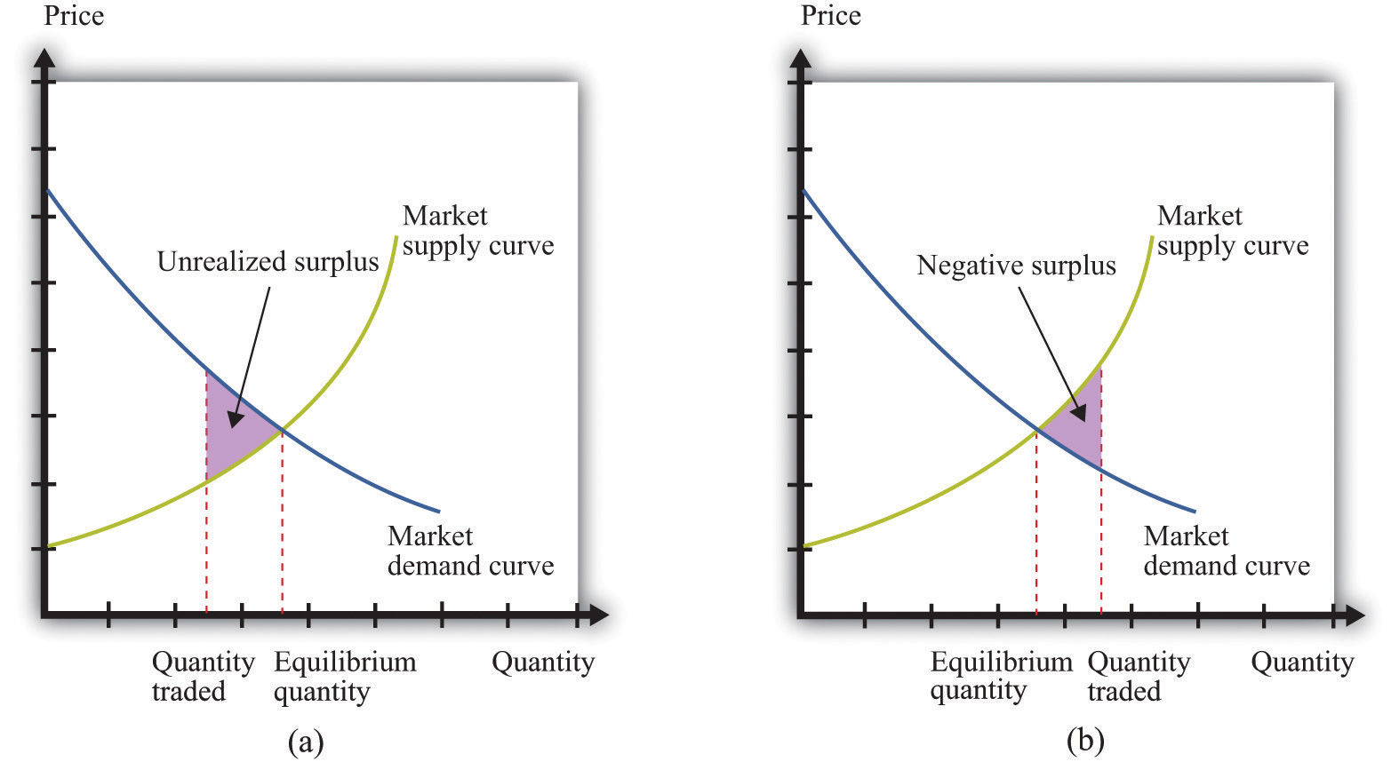
If the quantity traded is less than the equilibrium quantity (a), then some gains from trade go unrealized. If the quantity traded is greater than the equilibrium quantity (b), then some trades generate negative surplus.
We have been highlighting one of the principal messages in economics: markets are a mechanism to achieve the gains from trade. But are there other ways of achieving the same result? We previously introduced the fiction of an all-knowing, all-powerful central planner. Such a planner tells everyone what they should produce, takes all those goods, and distributes them throughout the economy. The planner tells everybody how much to work at each technology and decides exactly how to distribute all the goods and services that the economy produces.
Should we take this idea seriously or is it only a device to help us think about our theory? The answer is a bit of both. No economy has ever literally been run by a central planner. Historically, though, there have been many examples of so-called planned economies, where government bureaucracies played a major role in deciding what goods and services should be produced. For much of the 20th century, the economy of the Soviet Union operated under such a regime. China also used to be a largely planned economy. North Korea still operates as a largely planned economy.
Neither the Soviet Union nor China enjoyed much economic success under this system. The collapse of the Soviet Union’s economy was a key reason why the country itself collapsed. China eventually changed its system of economic organization to one that gives more primacy to markets. Today, there are very few economies that operate under central planning and none that are significant in global economic terms. However, there are still several economies in which the government plays a significant role in the allocation of resources; so the analysis of the planner remains relevant.
Why were planned economies so unsuccessful? Books have been written on this topic, but there is one key insight. In order to make good decisions—decisions in the interest of individuals in the economy—the planner would need a lot of information. It is simply inconceivable that a planner could have sufficient knowledge about the abilities and skills of different individuals to make good decisions about where and how much they should work. Moreover, the planner also needs to know the tastes of everyone in the economy. Without that knowledge, the planner might instruct them to produce too many chocolate bars or not enough beer. If we think of an economy with millions of inhabitants, all with their own preferences and abilities, it is surely impossible that a planner could be sufficiently well informed to make decisions that are in the interest of all an economy’s inhabitants.
In other chapters in this book, we use the supply-and-demand framework to look at how goods and services are traded.We focus on labor in Chapter 8 "Growing Jobs" and Chapter 10 "Raising the Wage Floor". Chapter 9 "Making and Losing Money on Wall Street" looks at both the loan/credit market and the foreign exchange market. Here we give a brief overview of these markets.
The credit market (or loan market)Where suppliers and demanders of credit meet and trade.—we use the terms loans and credit interchangeably—is where suppliers and demanders of credit meet and trade (Figure 7.16 "Credit Market Equilibrium"). On the supply side are households and firms that, for various reasons, have chosen to save some of their current income. On the demand side are other households, firms, and (in some cases) the government. Households buy houses and cars, so they often need to borrow funds to finance those purchases. Firms seek credit to finance investment, such as the construction of a new production plant. Finally, governments borrow to finance some of their expenditures.
Figure 7.16 Credit Market Equilibrium
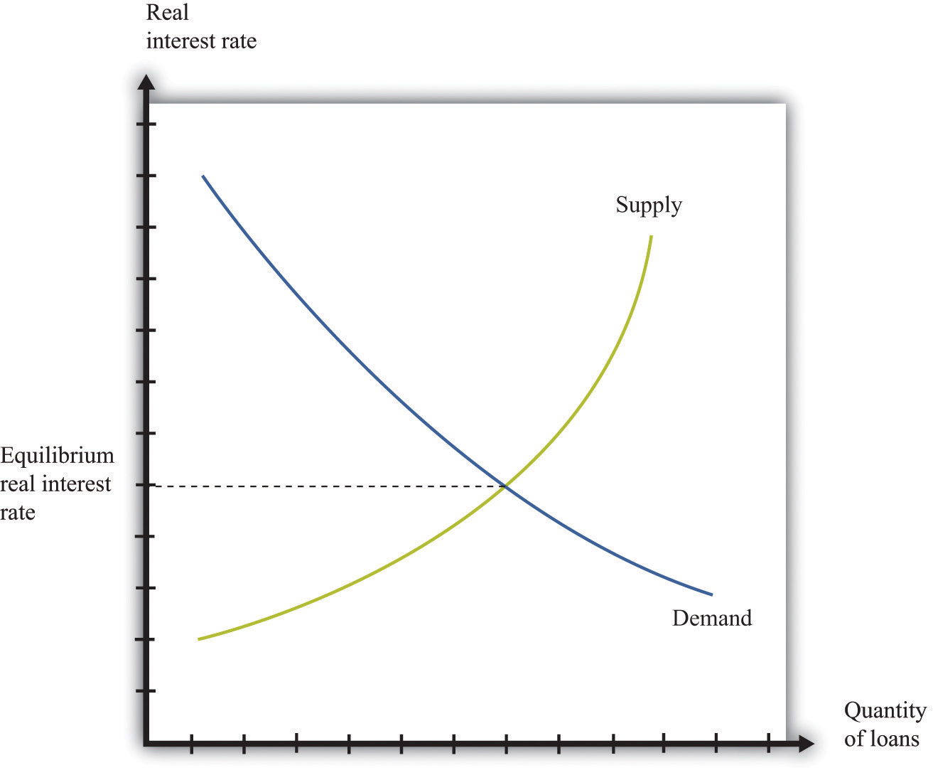
This diagram represents the loan or credit market.
The price of credit is the real interest rate, which is a measure of the value of the interest charged on a loan, adjusted for inflation. There are many different markets for credit because there are different kinds of loans in the economy.Chapter 9 "Making and Losing Money on Wall Street" discusses these. Associated with these different credit markets are different interest rates. For simplicity, though, we often suppose that there is a single market for credit.
Toolkit: Section 17.6 "The Credit Market"
You can review the credit market and the real interest rate in the toolkit.
The demand for credit decreases as the real interest rate increases. When it becomes more expensive to borrow, households, firms, and even governments want fewer loans. The supply of credit by households increases with the real interest rate. When the return on savings increases, households and firms will typically save more and so supply more loans to the market.The response of savings to changes in the real interest rate is discussed more fully in Chapter 4 "Life Decisions".
The news is filled with stories about interest rates increasing and decreasing. You can always use some version of Figure 7.16 "Credit Market Equilibrium" to understand why interest rates are changing. Ultimately, any change in the interest rate is due to a shift in either the supply of credit or the demand for credit. For example, if construction firms anticipate high future demand for housing, they will think that building new homes is a good use of investment funds. They will borrow to finance such construction. The increased demand for credit will shift the demand curve in Figure 7.16 "Credit Market Equilibrium" outward, and interest rates will increase. As another example, if individuals in other countries wish to increase their investment in US assets, this will shift the supply of credit outward, and interest rates will decrease.
Two of the most important players in the credit market are the government and the monetary authority. If the US federal government borrows more, this shifts the demand for credit outward and increases the interest rate. (The government is such a big player in this market that its actions affect the interest rate.) The monetary authority, meanwhile, buys and sells in credit markets to influence the real interest rate in the economy.The actions of the Federal Reserve and other monetary authorities are studied in detail in macroeconomics courses.
If you travel abroad, you need to acquire the currency used in that region of the world. If you take a trip to Finland, Russia, and China, for example, you will undoubtedly buy euros, rubles, and yuan along the way. To do so, you need to participate in the foreign exchange marketThe place where suppliers and demanders of currencies meet and trade., trading one currency for another. Foreign exchange markets operate like other markets in the economy. The price—which in this case is called the exchange rateThe price in the foreign exchange market. It measures the price of one currency in terms of another.—is determined by the interaction of supply and demand.
Toolkit: Section 17.20 "Foreign Exchange Market"
The foreign exchange market is the market where currencies are traded. The price in this market is the price of one currency in terms of another and is called the exchange rate.
Figure 7.17 "Foreign Exchange Market Equilibrium" shows an example of a foreign exchange market—the market in which US dollars are exchanged for euros. On the horizontal axis, we show the number of euros bought and sold on a particular day. On the vertical axis is the exchange rate: the price of euros in dollars. This market determines the dollar price of euros just like the gasoline market in the United States determines the dollar price of gasoline.
Figure 7.17 Foreign Exchange Market Equilibrium
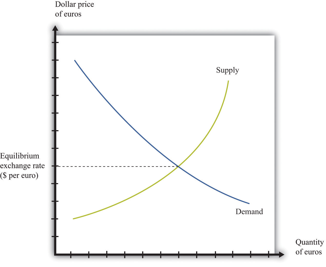
This diagram represents the foreign exchange market in which euros are bought and sold with US dollars.
On the demand side, there are traders (households and firms) who want to buy European goods and services. To do so, they need to buy euros. This demand for euros expressed in dollars need not come from US households and firms. Anyone holding dollars is free to purchase euros in this market. On the supply side, there are also traders (households and firms) who are holding euros and who wish to buy US goods and services. They need to sell euros to obtain US dollars.
There is another source of the demand for and the supply of different currencies. Households and, more importantly, firms often hold assets denominated in different currencies. You could, if you wish, hold some of your wealth in Israeli government bonds, in shares of a South African firm, or in Argentine real estate. But to do so, you would need to buy Israeli shekels, South African rand, or Argentine pesos. Likewise, many foreign investors hold US assets, such as shares in Dell Computer or debt issued by the US government. Thus the demand and the supply for currencies are influenced by the portfolio choices of households and firms. In practice, the vast majority of trades in foreign exchange markets are conducted by banks and other financial institutions that are adjusting their asset allocation.
In addition to households and firms, monetary authorities also participate in foreign exchange markets. For example, the US Federal Reserve Bank monitors the value of the dollar and may even intervene in the market, buying or selling dollars in an attempt to influence the exchange rate.
If you open a newspaper or browse the Internet, you can quickly find the current price of euros. This price changes all the time in response to changes in the currency’s demand and supply. For example, if you read that the euro is getting stronger, this means that the euro is becoming more expensive: you must give up more dollars to buy a euro. This increase in the price of the euro could reflect either an outward shift in the demand for euros, say as US households demand more goods from Europe, or an inward shift of the euro supply curve if holders of euros are not as willing to sell them for dollars.
In the markets for goods and services, the supply side usually comes from firms. In some cases, buyers are other firms (businesspeople call these B2B transactions), whereas in other cases buyers are households (often called B2C transactions). For the most part, though, households are not on the supply side of these markets. In the labor market, by contrast, firms and households switch roles: firms demand labor and households supply it.
Supply and demand curves for labor are shown in Figure 7.18 "Labor Market Equilibrium". Here the price of labor is the real wage. The real wage measures how much in the way of goods and services an individual can buy in exchange for an hour’s work. It equals the nominal wage (the wage in dollars) divided by the general price level.
Toolkit: Section 17.3 "The Labor Market"
You can review the labor market and the real wage in the toolkit.
The demand for labor comes from the fact that workers’ time is an input into the production process. This demand curve obeys the law of demand: as the price of labor increases, the demand for labor decreases. The supply of labor comes from households that allocate their time between work and leisure activities. In Figure 7.18 "Labor Market Equilibrium", the supply of labor is upward sloping. As real wage increases, households supply more labor. There are two reasons for this: (1) higher wages induce people to work longer hours, and (2) higher wages induce more people to enter the labor force and look for a job.Chapter 10 "Raising the Wage Floor" explains more about nominal wages and real wages, and we study the individual demand for labor in Chapter 8 "Growing Jobs". The decisions underlying labor supply are explained more fully in Chapter 3 "Everyday Decisions".
Figure 7.18 Labor Market Equilibrium
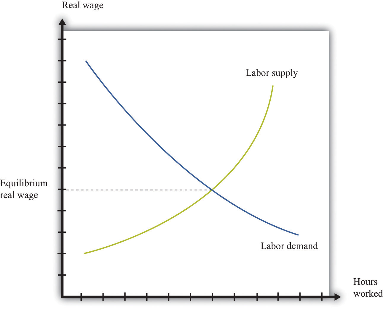
The equilibrium real wage is the price where supply equals demand in the labor market.
As with the other markets, we can use Figure 7.18 "Labor Market Equilibrium" to study comparative statics. For example, if an economy enters a boom, firms see more demand for their products, so they want to buy more labor to produce more product. This shifts the labor demand curve outward, with the result that real wages increase and employment is higher.
You have now seen equilibrium in a wide variety of markets: goods (chocolate), loans, foreign exchange, and labor. Actual economies contain hundreds of thousands of markets. Analyzing a single market would be enough if the markets in an economy were not connected, but markets are interrelated in many ways:A topic in advanced studies of economics is the simultaneous equilibrium of all markets. Because all markets are linked, it is necessary to find prices for all goods and services and all inputs simultaneously such that supply equals demand in all markets. This is an abstract exercise and uses lots of mathematics. The bottom line is good news: we can usually expect an equilibrium for all markets.
The following newspaper story from the Singaporean newspaper the Straits Times nicely illustrates linkages across markets.
Singaporeans with a sweet tooth could soon find themselves paying more for their favourite treats, as bakers and confectioners buckle under soaring sugar prices.
Since March last year, the price of white sugar has shot up by 70 per cent, according to the New York Board of Trade. As if that didn’t make life difficult enough for bakers, butter and cheese prices have also risen, by 31 per cent and 17 per cent respectively.
The increases have been caused by various factors: a steep drop in Thailand’s sugarcane production due to drought, higher sea freight charges, increasing demand from China’s consumers for dairy products and the strong Australian and New Zealand dollar.See http://straitstimes.asia1.com.sg. We also discuss this quote in Chapter 5 "eBay and craigslist".
Look at the last paragraph. First, we are told that a drought has caused a drop in sugarcane production in Thailand. Part (a) of Figure 7.19 "The Sugar Market in Thailand and the Butter Market in Australia" shows this market. We can see that a decrease in sugar production will increase the price of sugar. In this picture we are showing the market in Thailand, so the price is measured in Thai baht.
Figure 7.19 The Sugar Market in Thailand and the Butter Market in Australia
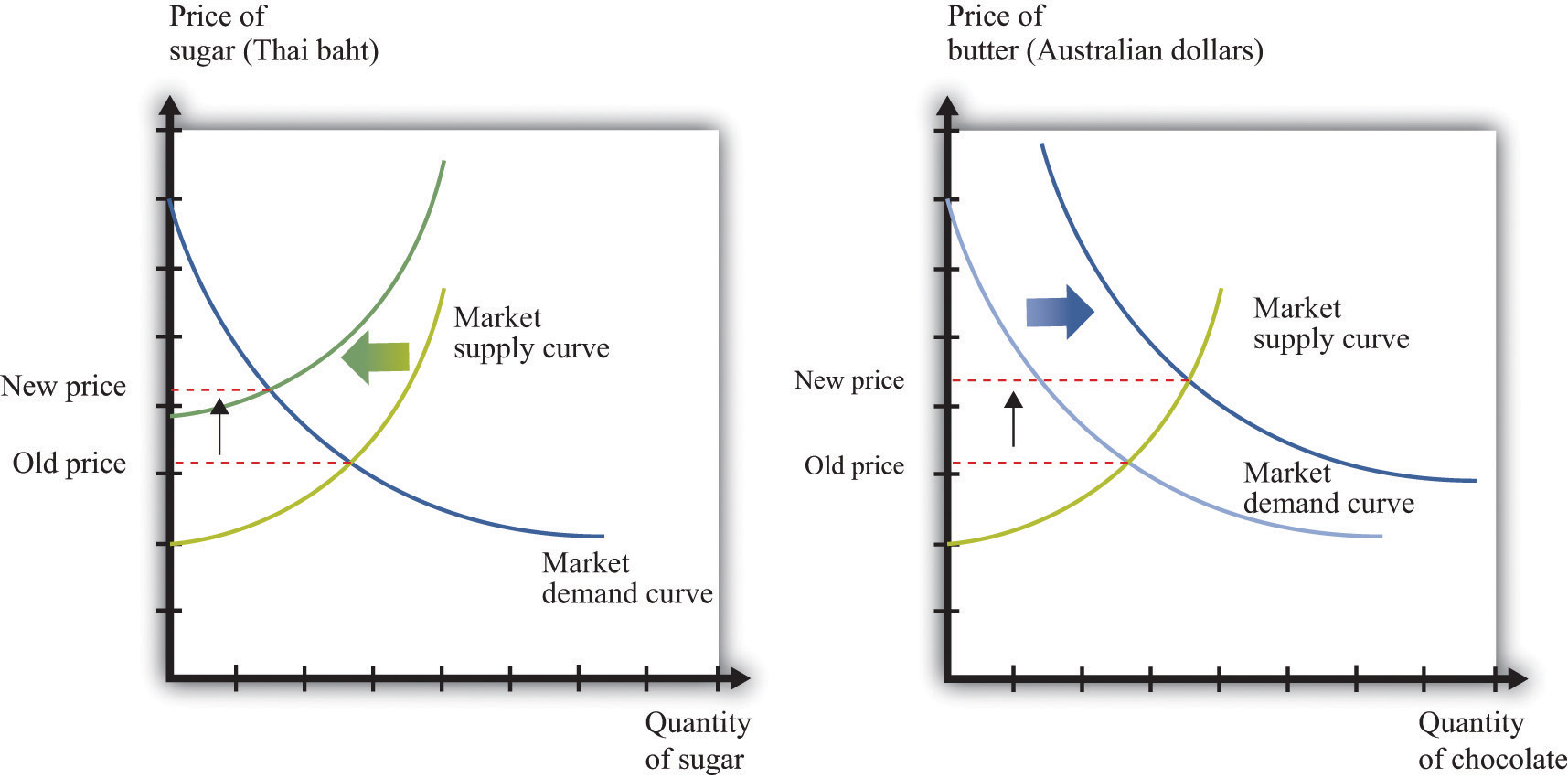
(a) The market for sugar in Thailand is affected by a drought, which has decreased the sugar supply, causing an increase in sugar prices measured in Thai baht. (b) In the Australian butter market, increased demand from China causes the demand curve to shift outward, increasing the price of butter measured in Australian dollars.
We are also told that there has been increased demand for dairy products coming from China. Australia and New Zealand are the major suppliers of dairy products in Southeast Asia. Part (b) of Figure 7.19 "The Sugar Market in Thailand and the Butter Market in Australia" shows the market for butter in Australia. Increased demand from China shifts the demand curve outward, leading to an increase in the price of butter. For this market, we measure the price in Australian dollars.
From the perspective of Singapore bakers, both of these price changes show up as increases in their marginal cost. Moreover, the article reveals that these changes are exacerbated by other factors. Shipping costs have increased, so it also costs more to obtain sugar from Thailand and butter from Australia. And the Australian dollar has appreciated relative to the Singapore dollar, making goods imported from Australia even more expensive.
These are examples of B2B transactions. In fact, there is likely a whole chain of such transactions between, say, the Australian dairy farmer and the Singaporean baker. Farmers sell milk to butter producers, butter producers sell to wholesalers, and wholesalers sell to Singaporean importers and bakeries.
This story also illustrates again the powerful way in which market prices provide information that helps us understand the efficient allocation of resources. Drought in Thailand has reduced the amount of sugar available in the world. Through the magic of a series of prices, one of the results is that people in Singapore are less likely to eat cake for dessert.
Everything that we have discussed in this chapter applies, strictly speaking, only to perfectly competitive markets. Yet the conditions for perfect competition are quite stringent. For a market to be perfectly competitive, there must be a large number of sellers of an identical product. There also must be a large number of buyers. Each buyer and seller must be “small” relative to the market, meaning that they cannot influence market price.
There are certainly some markets that fit these criteria. Markets for commodities, such as wheat or gold, are one example. Markets for certain financial assets are another. Such examples notwithstanding, the vast majority of markets are not perfectly competitive. In most markets, firms possess some market power, meaning that the demand curve they face is not perfectly elastic.
You might think this greatly weakens the usefulness of the supply-and-demand framework. A firm with market power chooses a point on the demand curve that it faces. It sets a price as a markup over marginal cost and then produces enough to meet demand at that price.We explain how firms set these prices in Chapter 6 "Where Do Prices Come From?". A firm with market power does not take the price as given and then determine a quantity to supply. In fact—strictly speaking—there is no such thing as a supply curve when a firm has market power.
Economists understand this very well. Yet suppose you ask an economist to predict the likely effect of a worsening conflict in the Middle East on oil prices. The mental model she will use is almost certainly to imagine a supply curve for oil shifting to the left. Based on this model, she will predict higher prices and lower consumption. If you were to ask another economist to predict the effects of an economic recession on purchases of automobiles, he would imagine a demand curve shifting to the left and thus predict lower prices and lower output.
The first economist would use a supply-and-demand framework even though oil producers have market power. The second economist would use a supply-and-demand framework even though not all cars are identical. Although economists understand that many markets do not satisfy the strict conditions of perfect competition, they also know that the intuition from comparative statics carries over to more general market structures.
To see why, let us go back to our beer example again. We all know that not all beer is the same, and the beer companies spend a lot of money to convince us of this fact. Different beers have different tastes, and there are customers who are loyal to different beer brands. Breweries possess market power, meaning that we cannot—strictly speaking—draw a supply curve for individual beer producers or for the market as a whole.
Yet our comparative statics story, which supposes that the beer market is competitive, gives us an answer that makes sense. When the price of hops increases, this increases the marginal cost of production for all beer producers. Because they set prices based on a markup over marginal cost, the price of beer will increase, and less will be consumed. Output will be lower for all producers, and prices will be higher. Our comparative statics technique gives the right answer. Let us go through this more formally, first for a change in production costs and then for a change in demand.
Figure 7.20 "Finding the Profit-Maximizing Price and Quantity When a Firm Has Market Power" shows how a firm with market power sets its price.This figure is explained more fully in Chapter 6 "Where Do Prices Come From?". To maximize its profits, a firm wants to produce the quantity where marginal revenue equals marginal cost. It sets the appropriate price as a markup over marginal cost.
Toolkit: Section 17.15 "Pricing with Market Power"
You can review the details of pricing with market power, including marginal revenue and markup, in the toolkit.
Figure 7.20 Finding the Profit-Maximizing Price and Quantity When a Firm Has Market Power
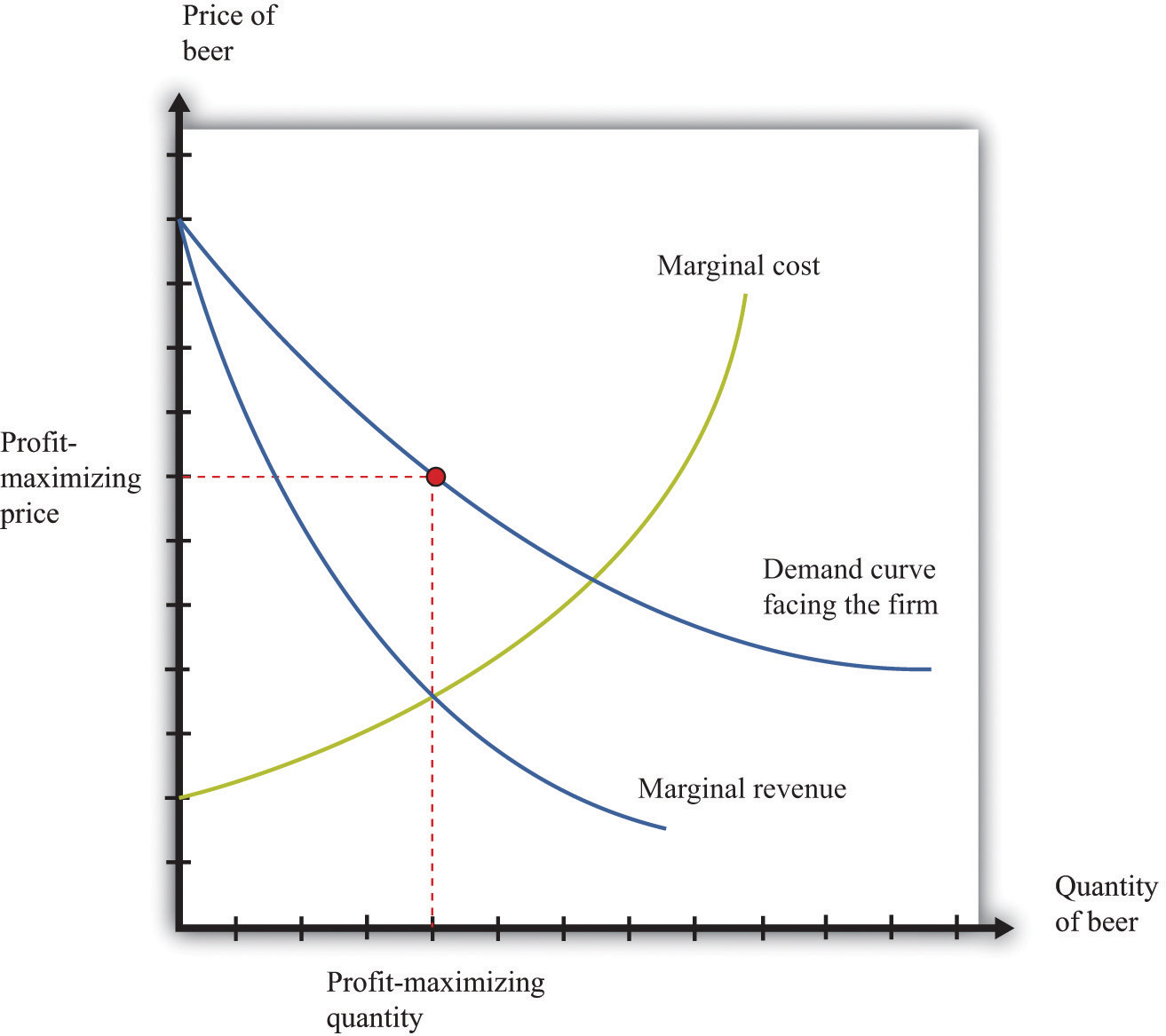
A firm with market power faces a downward-sloping demand curve and earns maximum profit at the point where marginal revenue equals marginal cost.
Now what happens if marginal cost increases? Think of a single beer producer and then imagine that the price of hops increases, so the marginal cost of producing an extra unit of output increases. This change in the marginal cost of production leads the brewer to decrease production (Figure 7.21 "An Increase in Marginal Cost"). Marginal cost decreases and marginal revenue increases until the two are again equal.
Figure 7.21 An Increase in Marginal Cost
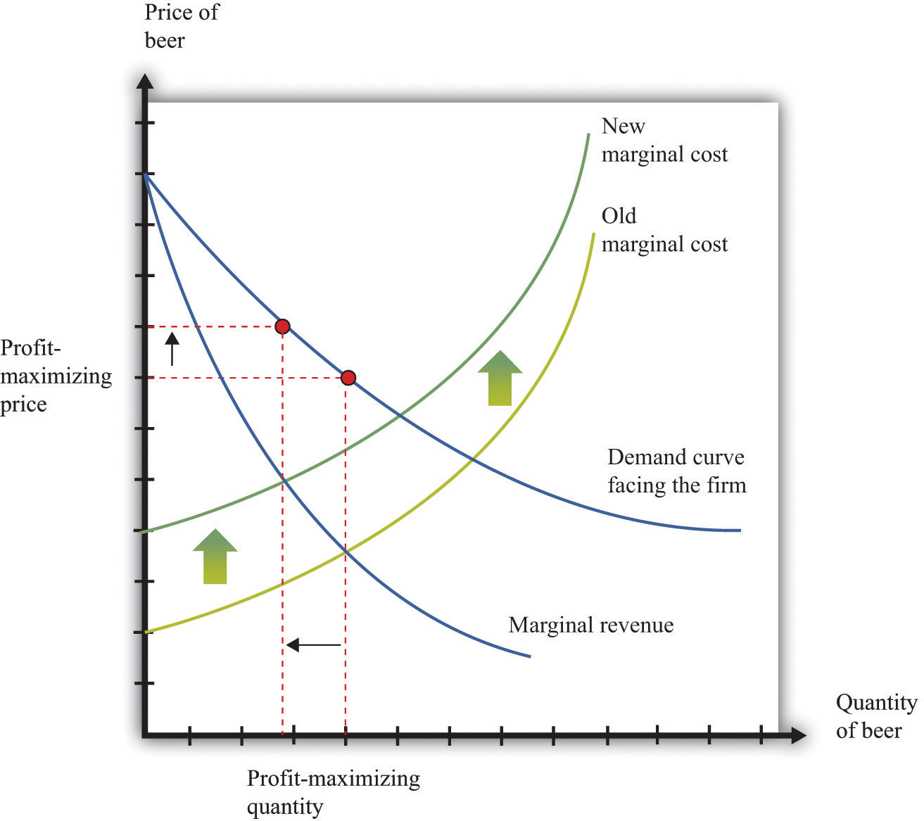
In response to an increase in marginal cost, a firm now finds it optimal to set a higher price and produce a smaller quantity of beer.
Although Figure 7.21 "An Increase in Marginal Cost" is drawn for a single seller, it captures the common experience and response of all sellers. The increase in the price of hops causes the marginal cost to increase for all brewers, and they all respond by producing less and increasing the price of beer. And this is exactly what we predicted about prices and quantities when we considered an increase in marginal cost in a perfectly competitive market.
Now reconsider the T-shirt example. There may be only a small number of producers who are licensed to produce Detroit Tigers T-shirts. Although there are many different kinds of replica sporting shirts in the world—at least one for each major team in most of the sports you can imagine—these shirts are not all the same. So the market for replica T-shirts—and certainly the market for Granderson T-shirts—is not competitive. The producers of Granderson shirts for the Tigers choose quantities and set prices (see Figure 7.20 "Finding the Profit-Maximizing Price and Quantity When a Firm Has Market Power").
Figure 7.22 "Shifts in Demand and Marginal Revenue" shows the market as seen by one of these producers. Granderson’s move from the Tigers shifts the demand curve inward for the shirts that they produce. This shift in the demand curve also shifts the marginal revenue curve inward. In response, the firm adjusts its output so that marginal revenue again equals marginal cost, choosing its price to match the point on the demand curve at the new quantity produced. Output and price both fall. Again, this is the same prediction that we obtained from the comparative statics of a competitive market.
Figure 7.22 Shifts in Demand and Marginal Revenue

A decrease in demand causes marginal revenue to shift to the left. Marginal cost and marginal revenue intersect at a lower level of output. This lower level of output means marginal cost is lower, so the firm will also decrease its price.
Even when markets are not perfectly competitive, the supply-and-demand framework is usually a good device for predicting what will happen to prices and quantities in a market following a shock. Even if firms have market power, an increase in marginal cost will typically lead to an increase in the price and a decrease in the quantity supplied, just as supply and demand predict. Similarly, an increase in demand will typically lead to an increase in the price and an increase in the quantity supplied, again as predicted by basic supply-and-demand reasoning.
Although the supply-and-demand framework can be used for most situations where markets are not perfectly competitive, we still need to know when it might mislead us.
We also need to recognize that while we may be able to use supply-and-demand intuition for qualitative predictions, it is more difficult to make quantitative predictions when markets are not competitive. We cannot determine supply and demand elasticities as easily when firms have market power. The reason is that one firm’s decisions depend on what other firms are doing. Consider, for example, an increase in marginal cost in the beer industry. We have said that each firm in the market will respond by increasing its price and decreasing its quantity (Figure 7.21 "An Increase in Marginal Cost"). For example, Miller in the United States will set higher prices in response to an increase in the price of hops. But when markets are not perfectly competitive, the story does not stop there. Firms also look at the prices set by their competitors. Miller’s decisions on pricing depend also on the price chosen by Budweiser. If Budweiser sets a higher price as well, then Miller may want to increase its price still further, and so on.How exactly this plays out is a complicated problem, requiring some of the ideas that we introduce in Chapter 14 "Busting Up Monopolies" and Chapter 16 "Cars".
To sum up, the supply-and-demand framework can occasionally mislead when markets are not perfectly competitive. Yet most economists still begin with supply and demand when trying to explain a change in prices or quantities. Then they consider if there are reasons to expect either changes in the elasticity of demand or decreasing marginal cost. If neither of these seems likely, then the simple intuition of supply and demand will almost certainly give the right answer.
The supply-and-demand framework is the most powerful framework in the economist’s toolkit. Armed with an understanding of this framework, you can make sense of much economic news, and you can make intelligent predictions about future changes in prices.
A true understanding of this framework is more than just an ability to shift curves around, however. It is an understanding of how markets and prices are one of the main ways in which the world is interlinked. Markets are, quite simply, at the heart of economic life. Markets are the means by which suppliers and demanders of goods and services can meet and exchange their wares. Because exchange creates value—it makes both buyers and sellers better off—markets are the means by which our economy can prosper. Markets are the means by which economic activity is coordinated in our economy, allowing us to specialize in what we do best and buy other goods and services.
Economists wax lyrical about these features of markets, but this should not blind us to the fact that markets can go wrong. There are many ways in which market outcomes may not be the most desirable or efficient. In other chapters, we look in considerable detail at all the ways that markets can fail us as well as help us.
Fill in the missing values in Table 7.5 "Individual and Market Demand". What can you say about the missing price in the table?
Table 7.5 Individual and Market Demand
| Price of Chocolate Bars ($) | Household 1 Demand | Household 2 Demand | Market Demand |
|---|---|---|---|
| 1 | 7 | 22 | |
| 2 | 11 | 16 | |
| 10 | 0.5 | 3 | 3.5 |
| 0.75 | 4 | 4.75 |
Spreadsheet Exercise
Economics Detective
The supply-and-demand framework can be analyzed with algebra. We start with supply and demand and then talk about market equilibrium. This presentation uses some notation rather than only words:
With this notation, we represent the demand curve as follows:
Equation 7.1
qd = αd – βdp + γdI.αd, βd, and γd are constants that characterize the effects of prices and income on the quantity demanded. With the restriction that βd > 0, the demand curve is downward sloping because an increase in p implies a reduction in the quantity demanded. It is natural to assume γd > 0, so an increase in income leads to an increase in the quantity demanded. This is represented as a shift in the demand curve.
With this notation, we represent the supply curve as follows:
Equation 7.2
qs = αs – βsp + γsA.αs, βs, and γs are constants that characterize the effects of prices and income on the quantity demanded. With the restriction that βs > 0, the supply curve is upward sloping because an increase in p leads to an increase in the quantity supplied by all firms. It is natural to assume γs > 0, so an increase in the productivity of the current technology leads to an increase in the quantity produced at a given price. This is represented as a shift in the supply curve.
The market is in equilibrium if there is a price and quantity combination, denoted (p*, q*) such that at the price p*, the quantity demanded, and the quantity supplied equal q*. Equilibrium is the simultaneous solution of supply and demand and can be found using the substitution method outlined in the toolkit.
Using qs = qd = q*, we can substitute Equation 7.2 into Equation 7.1 yielding:
Equation 7.3
αd – βdp* + γdI = αs – βsp* + γsA.This is a single equation in a single unknown, p*. Solving the equation for p* implies
Equation 7.4
The denominator is positive because we have assumed that both βd and βs are positive. The numerator is positive as long as the vertical intercept of the demand curve is greater than the vertical intercept of the supply curve: (αd + γsI) > (αs + γdA). This condition, combined with the restrictions on the slopes of supply and demand, is sufficient to guarantee that an equilibrium price exists in the market.
Using this calculation of p* in, say, the supply curve, we find
Equation 7.5
Grouping the terms into a constant, γdI and γsA, this becomes
Equation 7.6
Looking at Equation 7.4 and Equation 7.6, these expressions determine the equilibrium price and the equilibrium quantity depending on the two (exogenous) factors that impact supply and demand: income level I and state of technology A. Though income influences only the position of the demand curve, variations in income influence both the equilibrium price and the equilibrium quantity. The same is true for variations in technology that shift only the supply curve.


