We have provided some facts about differences in income across households. We now turn to a discussion of where those differences come from.
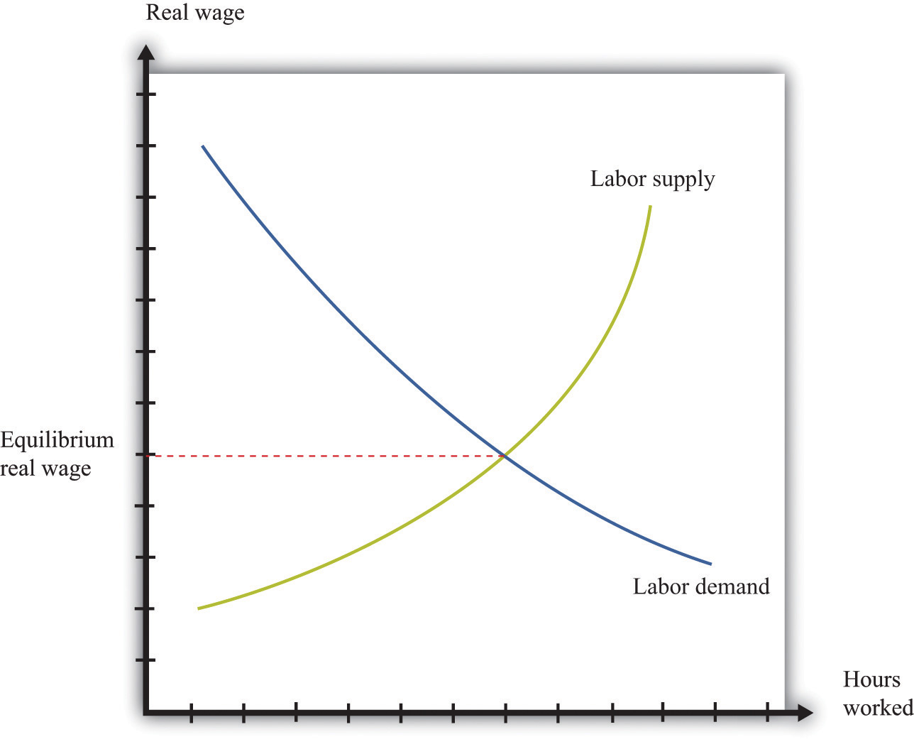
We begin by looking at earnings, by which we mean the income that households obtain from their work in the labor marketWhere suppliers and demanders of labor meet and trade.. Figure 12.5 "Labor Market Equilibrium" shows the labor market. The real wageThe nominal wage (the wage in dollars) divided by the price level. is on the vertical axis, and the number of hours worked is on the horizontal axis. The labor demand curve indicates the quantity of labor demanded by firms at a given real wage. As the real wage increases, firms demand less labor. The labor supply curve shows the total amount of labor households want to supply at a given real wage. As the real wage increases, the quantity of labor supplied also increases.See Chapter 3 "Everyday Decisions", Chapter 7 "Why Do Prices Change?", and Chapter 8 "Growing Jobs" for more discussion. Here we are interested in what the labor market can tell us about how much people earn.
Toolkit: Section 17.3 "The Labor Market"
You can find more details about the labor market in the toolkit.
Figure 12.5 Labor Market Equilibrium
When firms are deciding how many hours of work to hire, they use this decision rule: hire until
real wage = marginal product of labor.The left side of this equation represents the cost of purchasing one more hour of work. The right side of this equation is the benefit to the firm of one more hour of work: the marginal product of labor is the extra output produced by the extra hour of work. If the marginal product is higher than the real wage, a firm can increase its profits by hiring more hours of work.
We use this equation as a starting point for thinking about distribution and inequality. Different individuals in the economy are paid different real wages. This reflects, among other things, the fact that there is not a single labor market in the economy. Rather, there are lots of different markets for different kinds of jobs: accountants, barbers, computer programmers, disc jockeys, and so on. We can imagine a diagram like Figure 12.5 "Labor Market Equilibrium" for each market. In all cases, the firms doing the hiring will want to follow the rule given by the equation. And if firms follow this hiring rule, then two individuals who earn different real wages must differ in terms of their marginal product. The worker who earns the higher wage is also the worker who is more productive.
But why would workers have different marginal products? One reason is that people differ in terms of their innate abilities. For any individual, we could come up with a long list of the skills and abilities that he or she is born with—natural talents. Some are good at mathematics, some are particularly strong, some are good at music, some are good at building things, some are very athletic, some are good at managing other people, and so on. Abilities that tend to make someone have a high marginal product allow that person to earn higher real wages. Differences in innate abilities, then, are the first explanation we can suggest for why there are differences in earnings when we look across individuals.
The possession of innate ability is not enough to guarantee someone a high marginal product; the market must value the individual’s talents as well. The demand for particular abilities or skills is high if they can be used to produce something that people want to buy. Think about a talented quarterback: his talents translate into an ability to draw paying customers to games, which in turn translates into a willingness to pay a lot for his labor. Or think about a skilled manager: her ability to make good business decisions translates into higher profits for a firm, which in turn translates into a willingness to pay for her labor. If an ability is valued in the market, then there will be high demand for the labor of people with that ability.
What is valuable changes over time and from place to place. Being a skilled quarterback is valued in the modern-day United States. The same innate talent was worth much less 50 years ago in the United States and is still worth little today in a village in the Amazon. Rock stars who can earn hundreds of millions of dollars today would have had very little earning power in 19th-century Australia. The same holds for more mundane skills. The innate abilities that make for a good software designer are more valuable than in the past; the innate abilities that make for a good clockmaker are less valuable than in the past.
Labor supply matters because the value of your innate abilities also depends on how many other people have similar talents. Another reason that highly talented quarterbacks command such high earnings is because their abilities are in short supply. Being a good taxi driver also requires certain skills, but these are much more common. As a result, the supply of taxi drivers is larger, so the real wage earned by taxi drivers is smaller.
Star quarterbacks have innate abilities that most of us don’t possess. But they also have more training and experience in this role. Just about every one of us could be a better quarterback than we are now, if we were willing to train several hours a day. Indeed, most occupations require some skills and training. Computer programmers must learn programming languages, engineers must learn differential equations, tennis players must learn how to play drop shots, and truck drivers must learn how to reverse an 18-wheeler.
As well as such specific skills, an individual’s general level of education is usually an indicator of his or her marginal productivity and hence the wage that can be earned. Basic literacy and numeracy are helpful—if perhaps not absolutely necessary—for nearly any job. A high school education typically makes an individual more productive; a college education even more so. So the distribution of labor income is affected by the distribution of education levels. People also learn on the job. Sometimes this is through formal training programs; sometimes it just comes from accumulating experience. Generally, older and more experienced workers earn higher wages.
Education and experience affect both labor demand and labor supply. More highly skilled workers are typically more valuable to firms, so the demand curve for such workers lies further to the right. At the same time, experienced and trained workers tend to be in more limited supply, so the supply curve lies further to the left. Both effects lead to a higher real wage. Just as a worker’s real wage depends on how valuable and scarce are her abilities, so also does it depend on how valuable and scarce are her education and training.
The influence of experience on earnings is a reminder of an observation that we made when discussing the data. Even in a world where everyone is identical in terms of abilities and education, we would expect to see some inequality in earnings and income simply because people are at different stages of life. Younger, inexperienced workers often earn less than older, experienced workers.
In recent years, economists have looked closely at the differences in wages among skilled and unskilled workers. Loosely speaking, skilled workers are more educated and in occupations that rely more on thinking than on doing. So for example, an accountant is termed a skilled worker, and a construction worker with only a high-school diploma is an unskilled worker. Data on wages suggest that the return to skill, as measured by the difference in wages between skilled and unskilled workers, has widened dramatically since the mid-1970s. Many economists think that this is an important part of the explanation for the increasing inequality in the United States.
One way to measure the increased return to skills is to look at the financial benefit of education, given that more educated workers are typically skilled rather than unskilled. Table 12.8 "Relationship between Education and Inequality in the United States" summarizes some evidence on the distributions of earnings, income, and wealth from 1998. The table indicates that there is a sizable earnings gap associated with education. According to this sample, completing high school increased earnings by nearly $20,000, and a college degree led to an additional $34,000 in average annual income. Education is an important factor contributing to inequality. One way to decrease inequality is to improve access to education.
Table 12.8 Relationship between Education and Inequality in the United States
| Education | Earnings | Income (1998 $) | Wealth |
|---|---|---|---|
| No high school | 14,705 | 21,824 | 78,548 |
| High school | 34,211 | 43,248 | 189,983 |
| College | 68,530 | 88,874 | 541,128 |
Source: Santiago Rodríguez, Javier Díaz-Giménez, Vincenzo Quadrini, and José-Víctor Ríos-Rull, “Updated Facts on the U.S. Distributions of Earnings, Income and Wealth,” Federal Reserve Bank of Minneapolis Quarterly Review, Summer 2002. Here earnings come from both labor and business activities. Income includes transfers.
So far we have said nothing about how hard people choose to work, in terms of either the number of hours they put in on the job or their level of effort while working. Those who are willing to work longer hours and put in more effort will typically obtain greater earnings.
Effort is a matter of individual choice. Some other factors that can influence your earnings are likewise under your own control. Training and education are largely a matter of choice: you can choose to go to college or take a job directly out of high school. By contrast, the abilities you are born with are, from your point of view, a matter of luck. We have more to say about this distinction later when we evaluate the fairness of the distribution of income.
Study after study indicates that the gender of a worker also influences real wages. Figure 12.6 "Labor Market Outcomes for Women" shows the wage gap and the participation rates for married women in the United States.We are grateful to Michelle Rendell for this figure. The discussion in this section is drawn in part from her PhD dissertation research. The participation rate for married women—the fraction of married women in the labor force—has increased from slightly above 20 percent in 1950 to about 70 percent in 2000. Meanwhile, the ratio of wages paid to married women relative to married men displays an interesting pattern over this period. From 1950 to 1980, the ratio fell from 65 percent to 60 percent—that is, the wages of married women fell relative to married men. Thereafter, the ratio rose substantially, to about 80 percent in 2000. At the end of the 20th century, in other words, married women were earning about four-fifths of the wages of married men.
Figure 12.6 Labor Market Outcomes for Women

Economists and other social scientists are interested in understanding these facts. What was the source of the increased participation in the labor force by women and what factors increased their wages relative to men? One tempting approach is to use a supply-and-demandA framework that explains and predicts the equilibrium price and equilibrium quantity of a good. diagram like Figure 12.5 "Labor Market Equilibrium", thinking specifically about women’s labor. For example, we could explain the overall shift between 1950 and 2000 by a rightward shift of the labor demand curve. A shift to the right in the demand curve increases the real wage. The higher real wage would also induce women to supply more hours: this is the corresponding movement along the labor supply curve. More women would be induced to move away from work at home and toward work in the market, given the higher return for market work. To explain the increase in women’s wages relative to men’s, we would need to see a larger increase in the demand for women’s labor than for men’s labor.
But this is a somewhat odd story. There is no reason to think that there should be a separate labor market for women and men. Women and men can and do perform the same jobs and thus compete in the same labor market. Any supply-and-demand explanation needs to be subtler. One possibility is that there has been a shift in the kinds of jobs that are most important in the economy and hence a shift in the kinds of skills needed. Suppose, for example, that women are more likely to be accountants than construction workers. A shift in labor demand toward accountancy and away from construction will increase wages in accountancy relative to construction work and will therefore increase women’s wages, on average, relative to men’s. Researchers looking closely at the data see some evidence of such effects when they look at wages and employment patterns across jobs that require different skills.
There is another, perhaps even more basic question: why are women’s wages consistently lower than men’s wages? Researchers have also devoted a great deal of effort to this problem, looking to see in particular if differences in education and skills can account for the difference in wages. Typically, these studies have found that such differences can explain some—but not all—of the gap between wages for men and women. The remaining difference in wages is very possibly due to discrimination in the labor market. If this is the case, then recent increases in women’s wages relative to men’s wages could be due to a reduction in discrimination.
Of course, women are not the only group that has been subject to discrimination in the labor market. In the United States, African Americans and other minority groups have suffered from discrimination. In many other countries, there are similarly different groups that have been unfairly punished in the labor market. Economists point out that supply and demand is actually a positive force for combating discrimination. Discrimination against women workers, for example, means that women are being paid less than their marginal product. Nondiscriminatory employers then have an incentive to hire these workers and make more profit, which in turn would tend to increase women’s wages.
Economic forces can mitigate discrimination, but this is not an argument that discrimination is not or cannot be a real problem. First of all, discriminatory attitudes might make employers incorrectly perceive that the marginal product of women (or other groups) is lower than it actually is. Second, even if employers are not actively discriminating against women, coworkers may be discriminatory, and this could lead to lower productivity among women in the workforce. Research in social psychology tells us that such discrimination—by employers or colleagues—can occur even if people have no explicit discriminatory intent.
There are some markets where compensation reflects ability in a very extreme way. These are often called winner-takes-all marketsThe person with the highest ability captures the whole market, and everyone else gets nothing.. In such a market, the person with the highest ability captures the whole market, and everyone else gets nothing. You can think of this as a race where the winner of the race gets all the prize money. The phrase winner takes all is not meant literally. The idea is more that a small number of people earn very large returns. Think, for example, of the professional golf or tennis circuits, where perhaps a few hundred people obtain the winnings from the tournaments—and the bulk of the winnings go to a small number of top players.
In these markets, we cannot assume that the wage equals the marginal product of labor. In a winner-takes-all market, you get a wage that depends not on your productivity in isolation but on how your productivity compares with that of others. If you are the most productive, you win the entire market.
Many markets have at least some aspects of a winner-takes-all market. Think of the market for rock musicians. If there were one group that everyone liked more than all the others, then that group would sell CDs and MP3s, give concerts, and completely dominate the music scene. Other groups would disappear. The actual music market is not this extreme. There are many groups who produce songs, give concerts, and so on. But there is a clear ranking between the first-class groups and the others. So even though there is not a single winner who takes all the market, there are a relatively small number of big winners who together take most of the market.
Why does the market for rock musicians have winner-takes-all characteristics? A good way to understand the phenomenon is to think about the market for musicians centuries ago—before recording technologies. Good musicians might still be rewarded well—perhaps they would play for the king or queen—but there was room for, relatively speaking, a large number of good musicians because each would be serving only a relatively small local market. Today, though, the very best musicians can record their music and sell it all around the world. A single group, at relatively low marginal cost, can serve a very large market. (This is particularly true for CDs or MP3 files. It is less true for concert appearances because these do not have such low marginal cost.)
In winner-takes-all markets, there is a very skewed distribution of income relative to ability. Small differences in ability can translate into substantial differences in income. Moreover, winner-takes-all forces may be becoming stronger as a result of technological advances. The most popular rock stars, sport stars, and movie stars are now worldwide celebrities. Lady Gaga is famous in Thailand and Toledo; Brad Pitt is known from Denver to Denmark. This is perhaps one reason the very rich are getting relatively richer.
We are interested not only in the distribution of income but also in the distribution of consumption and wealth. To connect these three, we use the following equation:See Chapter 4 "Life Decisions" for more discussion.
wealth next year = (wealth this year + income this year − consumption this year) × interest factor.The first term on the right-hand side is the wealth you have at the start of a given year. To this wealth you add the income you earn in the current year and subtract your consumption. Because income − consumption = savings, this is the same as saying that you add your savings to your wealth. You earn interest income on your existing wealth and your new savings. Your initial wealth plus your savings plus your interest income gives you the wealth you can take into next year.
Suppose you currently have $1,000 in the bank. This is your wealth this year. You receive income of $300 and spend $200 of this income. This means that you save $100 of your income. So wealth this year plus income this year minus consumption this year equals $1,100. With an interest rate of 5 percent, your wealth next year would be $1,100 × 1.05 = $1,155.
This equation tells us several things.
The equation also conceals at least one relevant fact for inequality: wealthier households typically enjoy higher returns on their wealth. The interest rate is not the same for all households. There are several reasons for this, such as the fact that richer individuals find it worthwhile—and can afford—to hire professionals to manage their portfolios of assets or the fact that richer people may be able to purchase assets that are riskier but offer higher returns on average. It is not surprising that, as we saw, the wealth distribution is more unequal than the income distribution.
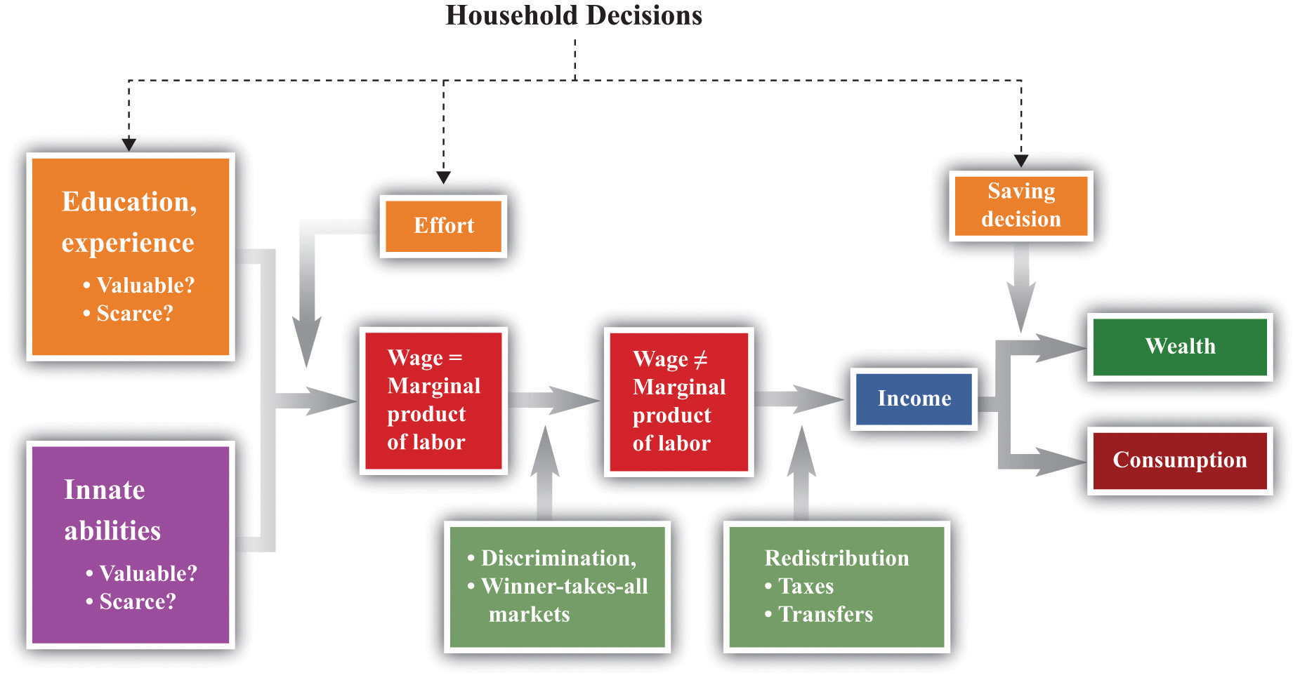
Figure 12.7 "The Different Sources of Inequality" brings together all the ideas we have discussed so far. It shows us three things. (1) Discrimination and winner-takes-all situations can break the simple link between the marginal product and the wage. (2) Government policies can break the simple link between wages and income. (3) Household decisions about how much to consume and save affect the observed amounts of income, consumption, and wealth. The figure also makes it clear that some of the forces leading to inequality are under the control of the individual, while others are outside the individual’s control.
Figure 12.7 The Different Sources of Inequality