By the end of this chapter, students should be able to:
Central banks have three primary tools for influencing the money supply: the reserve requirement, discount loans, and open market operations. The first works through the money multiplier, constraining multiple deposit expansion the larger it becomes. Central banks today rarely use it because most banks work around reserve requirements. (That is not to say that reserve requirements are not enforced, merely that they are not adjusted to influence MS. Currently, the reserve requirement is 10 percent on transaction account deposits [demand, ATS, NOW, and share draft] greater than $58.8 million.www.federalreserve.gov/monetarypolicy/reservereq.htm#table1) The second and third tools influence the monetary base (MB = C + R). Discount loans depend on banks (or nonbank borrowers, where applicable) first borrowing from, then repaying loans to, the central bank, which therefore does not have precise control over MB. Open market operations (OMO) are generally preferred as a policy tool because the central bank can easily expand or contract MB to a precise level. Using OMO, central banks can also reverse mistakes quickly.
In the United States, under typical conditions, the Fed conducts monetary policy primarily through the federal funds (fed funds) market, an overnight market where banks that need reserves can borrow them from banks that hold reserves they don’t need. Banks can also borrow their reserves directly from the Fed, but, except during crises, most prefer not to because the Fed’s discount rate is generally higher than the federal funds rate. Also, borrowing too much, too often from the Fed can induce increased regulatory scrutiny. So usually banks get their overnight funds from the fed funds market, which, as Figure 16.1 "Equilibrium in the fed funds market" shows, pretty much works like any other market.
Figure 16.1 Equilibrium in the fed funds market
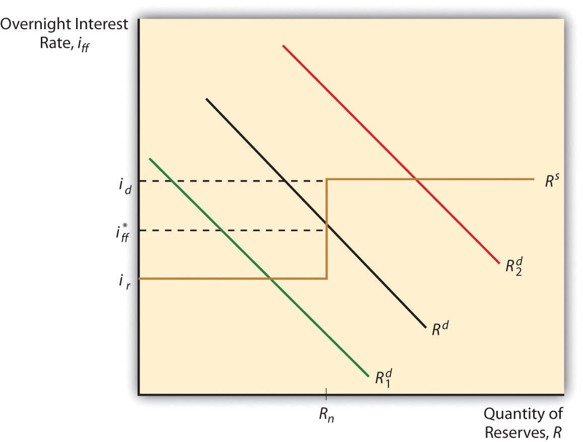
The downward slope of the demand curve for reserves is easily explained. Like anything else, as the price of reserves (in this case, the interest rate paid for them) increases, the quantity demanded decreases. As reserves get cheaper, banks will want more of them because the opportunity cost of that added protection, of that added liquidity, is lower. But what is the deal with that weird S-looking reserve supply curve? Note that the curve takes a hard right (becomes infinitely elastic) at the discount rate. That’s because, if the federal funds rate ever exceeded the discount rate, banks’ thirst for Fed discount loans would be unquenchable because a clear arbitrage opportunity would exist: borrow at the discount rate and relend at the higher market rate. Below that point, the reserve supply curve is vertical (perfectly inelastic) down to the rate at which the Fed pays interest on reserves (it currently pays .25% on both required and excess reserves, a practice begun in October 2008).www.federalreserve.gov/monetarypolicy/reqresbalances.htm Banks are, of course, unwilling to lend in the federal funds market at a rate below what the Fed will pay it, so the curve again becomes flat (infinitely elastic).
The intersection of the supply and demand curves is the equilibrium or market rate, the actual federal funds rate, ff*. When the Fed makes open market purchases, the supply of reserves shifts right, lowering ff* (ceteris paribus). When it sells, it moves the reserve supply curve left, increasing ff*, all else constant. In most circumstances, the discount and reserve rates effectively channel the market federal funds rate into a range.
Figure 16.2 Fed funds targeting, 2000–2010

Figure 16.3 Fed funds targeting, 2008
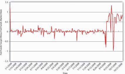
Theoretically, the Fed could also directly affect the demand for reserves by changing the reserve requirement. If it increased (decreased) rr, demand for reserves would shift up (down), increasing (decreasing) ff*. As noted above, however, banks these days can so easily sidestep required reserves that the Fed’s ability to influence the demand for reserves is extremely limited. Demand for reserves (excess reserves that is) can also shift right or left due to bank liquidity management activities, increasing (decreasing) as expectations of net deposit outflows increase (decrease). The Fed tries to anticipate such shifts and generally has done a good job of counteracting changes in excess reserves through OMO. Going into holidays, for example, banks often hold a little extra vault cash (a form of reserves). Knowing this, the Fed counteracts the rightward shift in demand (which would increase ff*) by shifting the reserve supply curve to the right by buying bonds (thereby decreasing ff* by an offsetting amount). Although there have been days when ff* differed from the target by several percentage points (several hundred basis points), between 1982 and 2007, the fed funds target was, on average, only .0340 of a percent lower than ff*. Between 2000 and the subprime mortgage uproar in the summer of 2007, the Fed did an even better job of moving ff* to its target, as Figure 16.2 "Fed funds targeting, 2000–2010" shows. During the crises of 2007 and 2008, however, the Fed often missed its target by a long way, as shown in Figure 16.3 "Fed funds targeting, 2008". So in December 2008, it stopped publishing a feds fund target and instead began to publish the upper limit it was willing to tolerate.
America’s first central banks, the BUS and SBUS, controlled commercial bank reserve levels by varying the speed and intensity by which it redeemed convertible bank liabilities (notes and deposits) for reserves (gold and silver). Can you model that system?
Kudos if you can! I’d plot quantity of reserves along the horizontal axis and interest rate along the vertical axis. The reserve supply curve was probably highly but not perfectly inelastic and the reserve demand curve sloped downward, of course. When the BUS or SBUS wanted to tighten monetary policy, it would return commercial bank monetary liabilities in a great rush, pushing the reserve demand curve to the right, thereby raising the interest rate. When it wanted to soften, it would dawdle before redeeming notes for gold and so forth, allowing the demand for reserves to move left, thereby decreasing the interest rate.
In practical terms, the Fed engages in two types of OMO, dynamic and defensive. As those names imply, it uses dynamic OMO to change the level of the MB, and defensive OMO to offset movements in other factors affecting MB, with an eye toward maintaining the federal funds target rate determined by the Federal Open Market Committee (FOMC) at its most recent meeting. If it wanted to increase the money supply, for example, it would buy bonds “dynamically.” If it wanted to keep the money supply stable but knew that a bank was going to repay a large discount loan (which has the effect of decreasing the MB), it would buy bonds “defensively.”
The responsibility for actually buying and selling government bonds devolves upon the Federal Reserve Bank of New York (FRBNY). Each trading day, FRBNY staff members look at the level of reserves, the fed funds target, the actual market fed funds rate, expectations regarding float, and Treasury activities. They also garner information about Treasury market conditions through conversations with so-called primary dealers, specialized firms and banks that make a marketBuying securities from all comers at a bid price and reselling them to all comers at a slightly higher ask price. in Treasuries. With the input and consent of the Monetary Affairs Division of the Board of Governors, the FRBNY determines how much to buy or sell and places the appropriate order on the Trading Room Automated Processing System (TRAPS) computer system that links all the primary dealers. The FRBNY then selects the best offers up to the amount it wants to buy or sell. It enters into two types of trades, so-called outright ones, where the bonds permanently join or leave the Fed’s balance sheet, and temporary ones, called repos and reverse repos. In a repo (aka a repurchase agreement), the Fed purchases government bonds with the guarantee that the sellers will repurchase them from the Fed, generally one to fifteen days hence. In a reverse repo (aka a matched sale-purchase transaction), the Fed sells securities and the buyer agrees to sell them to the Fed again in the near future. The availability of such self-reversing contracts and the liquidity of the government bond market render open market operations a precise tool for implementing the Fed’s monetary policy.
The so-called discount window, where banks come to borrow reserves from the Federal district banks, is today primarily a backup facility used during crises, when the federal funds market might not function effectively. As noted above, the discount rate puts an effective cap on ff* by providing banks with an alternative source of reserves (see Figure 16.4 "The discount window sets an upper bound on overnight interest rates"). Note that no matter how far the reserve demand curve shifts to the right, once it reaches the discount rate, it merely slides along it.
Figure 16.4 The discount window sets an upper bound on overnight interest rates
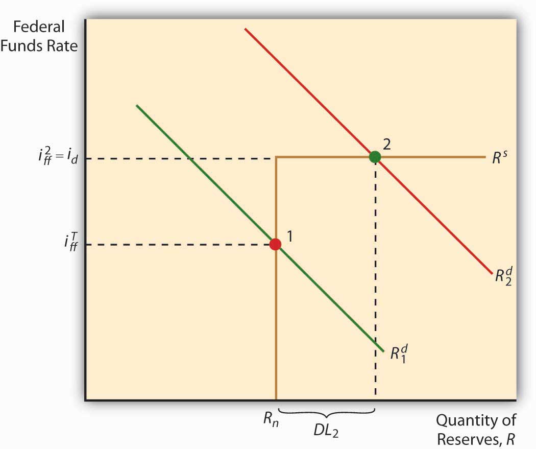
As lender of last resort, the Fed has a responsibility to ensure that banks can obtain as much as they want to borrow provided they can post what in normal times would be considered good collateral security. So that banks do not rely too heavily on the discount window, the discount rate is usually set a full percentage point above ff*, a “penalty” of 100 basis points. (This policy is usually known as Bagehot’s Law, but the insight actually originated with Alexander Hamilton, America’s first Treasury secretary, so I like to call it Hamilton’s Law.) On several occasions (including the 1984 failure of Continental Illinois, a large commercial bank; the stock market crash of 1987; and the subprime mortgage debacle of 2007), the discount window added the liquidity (reserves) and confidence necessary to stave off more serious disruptions to the economy.
Only depository institutions can borrow from the Fed’s discount window. During the financial crisis of 2008, however, many other types of financial institutions, including broker-dealers and money market funds, also encountered significant difficulties due to the breakdown of many credit markets. The Federal Reserve responded by invoking its emergency powers to create additional lending powers and programs, including the following:www.federalreserve.gov/monetarypolicy
Most of these programsblogs.wsj.com/economics/2011/08/09/a-look-inside-the-feds-balance-sheet-12/tab/interactive phased out as credit conditions returned to normal. (The Bank of England and other central banks have implemented similar programs.“Credit Markets: A Lifeline for Banks. The Bank of England’s Bold Initiative Should Calm Frayed Financial Nerves,” The Economist, April 26, 2008, 74–75.)
The financial crisis also induced the Fed to engage in several rounds of “quantitative easing” or Large Scale Asset Purchases (LSAP), the goals of which appear to be to increase the prices of (decrease the yields of) Treasury bonds and the other financial assets purchased and to influence the money supply directly. Due to LSAP, the Fed’s balance sheet swelled from less than a trillion dollars in early 2008 to almost 3 trillion by August 2011.
What in Sam Hill happened in Figure 16.5 "Total bank borrowings from the Federal Reserve System, 2001"? (Hint: The dates are important.)
Figure 16.5 Total bank borrowings from the Federal Reserve System, 2001
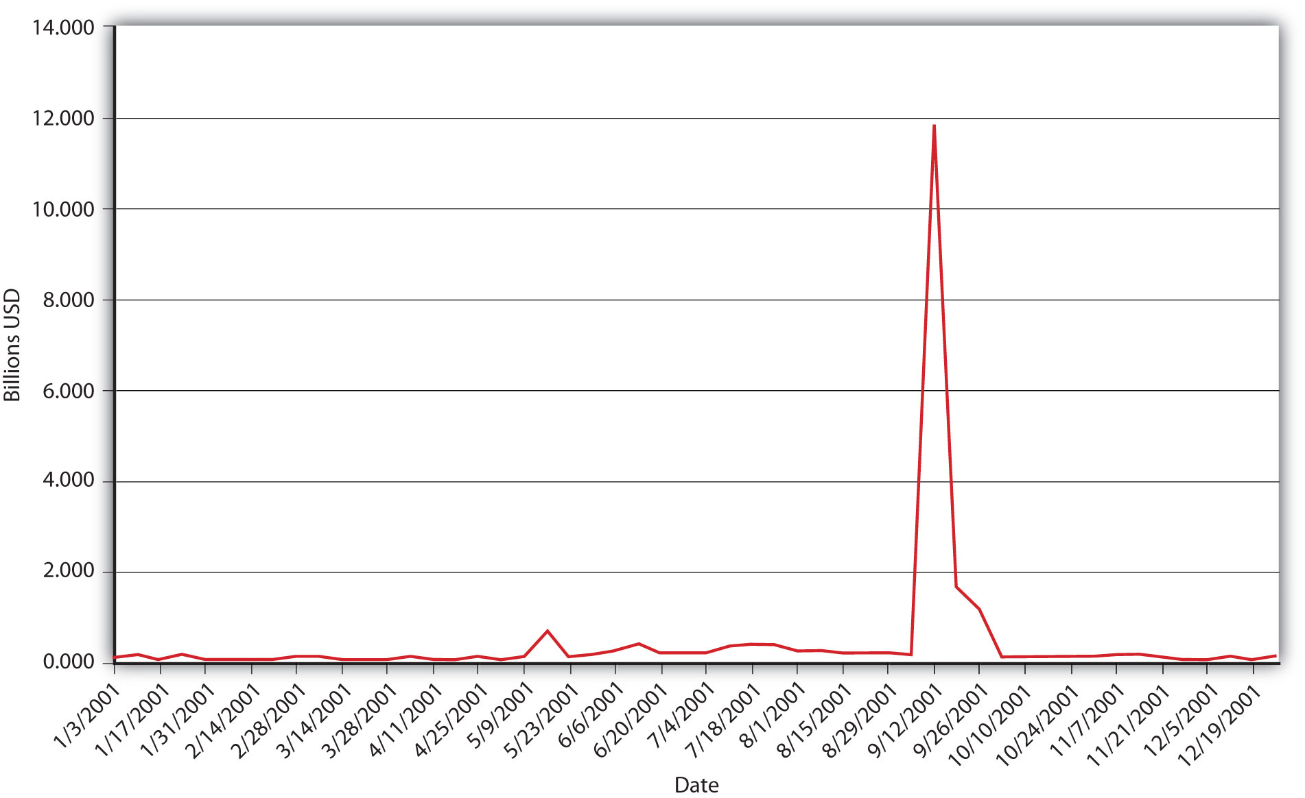
Terrorists attacked New York City and Washington, DC, with hijacked airplanes, shutting down the nation and parts of the financial system for the better part of a week. Some primary dealers were destroyed in the attacks, which also brought on widespread fears of bankruptcies and bank runs. Banks beefed up reserves by selling bonds to the Fed and by borrowing from its discount window. (Excess reserves jumped from a long-term average of around $1 billion to $19 billion.) This is an excellent example of the discount window providing lender-of-last-resort services to the economy.
The discount window is also used to provide moderately shaky banks a longer-term source of credit at an even higher penalty rate .5 percentage (50 basis) points above the regular discount rate. Finally, the Fed will also lend to a small number of banks in vacation and agricultural areas that experience large deposit fluctuations over the course of a year. Increasingly, however, such banks are becoming part of larger banks with more stable deposit profiles, or they handle their liquidity management using the market for negotiable certificates of deposit NCDs or other market borrowings.
The European Central Bank (ECB) also uses open market operations to move the market for overnight interbank lending toward its target. It too uses repos and reverse repos for reversible, defensive OMO and outright purchases for permanent additions to MB. Unlike the Fed, however, the ECB spreads the love around, conducting OMO in multiple cities throughout the European Union. The ECB’s national central banks (NCBs,) like the Fed’s district banks, also lend to banks at a so-called marginal lending rate, which is generally set 100 basis points above the overnight cash rate. The ECB pays interest on reserves, a central bank best practicePolicies generally considered to be state of the art in a given industry, to be something that nonconforming organizations ought to emulate. the Fed took up only recently.
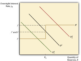
Canada, New Zealand, and Australia do likewise and have eliminated reserve requirements, relying instead on what is called the channel, or corridor, system. As Figure 16.6 "Paying interest on reserves puts a floor under the overnight interest rate" depicts, the supply curve in the corridor system looks like a weird S. The vertical part of the supply curve represents the area in which the central bank engages in OMO to influence the market rate, i*, to meet its target rate, it. The top horizontal part of the supply curve, il for the Lombard rate, is the functional equivalent of the discount rate in the American system. The ECB and other central banks using this system, like the Fed, will lend at this rate whatever amount banks with good collateral desire to borrow. Under normal circumstances, that quantity is nil because it (and i*) will be 25, 50, or more basis points lower, depending on the country. The big innovation in the channel system is the lower horizontal part of the supply curve, ir, or the rate at which the central bank pays banks to hold reserves. That sets a floor on i* because no bank would lend in the relatively risky overnight market if it could earn a safer, higher return by depositing its excess funds with the central bank. Using the corridor system, a central bank can keep the overnight rate within the bands set by il and ir and use OMO to keep i* near it.
Figure 16.6 Paying interest on reserves puts a floor under the overnight interest rate
Axilrod, Stephen H. Inside the Fed: Monetary Policy and Its Management, Martin Through Greenspan to Bernanke. Cambridge, MA: MIT Press, 2009.
Hetzel, Robert L. The Monetary Policy of the Federal Reserve: A History. New York: Cambridge University Press, 2008.
Mishkin, Frederic S. Monetary Policy Strategy. Cambridge, MA: MIT Press, 2007.