In macroeconomics, we seek to understand two types of equilibria, one corresponding to the short run and the other corresponding to the long run. The short runIn macroeconomic analysis, a period in which wages and some other prices are sticky and do not respond to changes in economic conditions. in macroeconomic analysis is a period in which wages and some other prices do not respond to changes in economic conditions. In certain markets, as economic conditions change, prices (including wages) may not adjust quickly enough to maintain equilibrium in these markets. A sticky priceA price that is slow to adjust to its equilibrium level, creating sustained periods of shortage or surplus. is a price that is slow to adjust to its equilibrium level, creating sustained periods of shortage or surplus. Wage and price stickiness prevent the economy from achieving its natural level of employment and its potential output. In contrast, the long runIn macroeconomic analysis, a period in which wages and prices are flexible. in macroeconomic analysis is a period in which wages and prices are flexible. In the long run, employment will move to its natural level and real GDP to potential.
We begin with a discussion of long-run macroeconomic equilibrium, because this type of equilibrium allows us to see the macroeconomy after full market adjustment has been achieved. In contrast, in the short run, price or wage stickiness is an obstacle to full adjustment. Why these deviations from the potential level of output occur and what the implications are for the macroeconomy will be discussed in the section on short-run macroeconomic equilibrium.
As we saw in a previous chapter, the natural level of employment occurs where the real wage adjusts so that the quantity of labor demanded equals the quantity of labor supplied. When the economy achieves its natural level of employment, it achieves its potential level of output. We will see that real GDP eventually moves to potential, because all wages and prices are assumed to be flexible in the long run.
The long-run aggregate supply (LRAS) curveA graphical representation that relates the level of output produced by firms to the price level in the long run. relates the level of output produced by firms to the price level in the long run. In Panel (b) of Figure 7.4 "Natural Employment and Long-Run Aggregate Supply", the long-run aggregate supply curve is a vertical line at the economy’s potential level of output. There is a single real wage at which employment reaches its natural level. In Panel (a) of Figure 7.4 "Natural Employment and Long-Run Aggregate Supply", only a real wage of ωe generates natural employment Le. The economy could, however, achieve this real wage with any of an infinitely large set of nominal wage and price-level combinations. Suppose, for example, that the equilibrium real wage (the ratio of wages to the price level) is 1.5. We could have that with a nominal wage level of 1.5 and a price level of 1.0, a nominal wage level of 1.65 and a price level of 1.1, a nominal wage level of 3.0 and a price level of 2.0, and so on.
Figure 7.4 Natural Employment and Long-Run Aggregate Supply
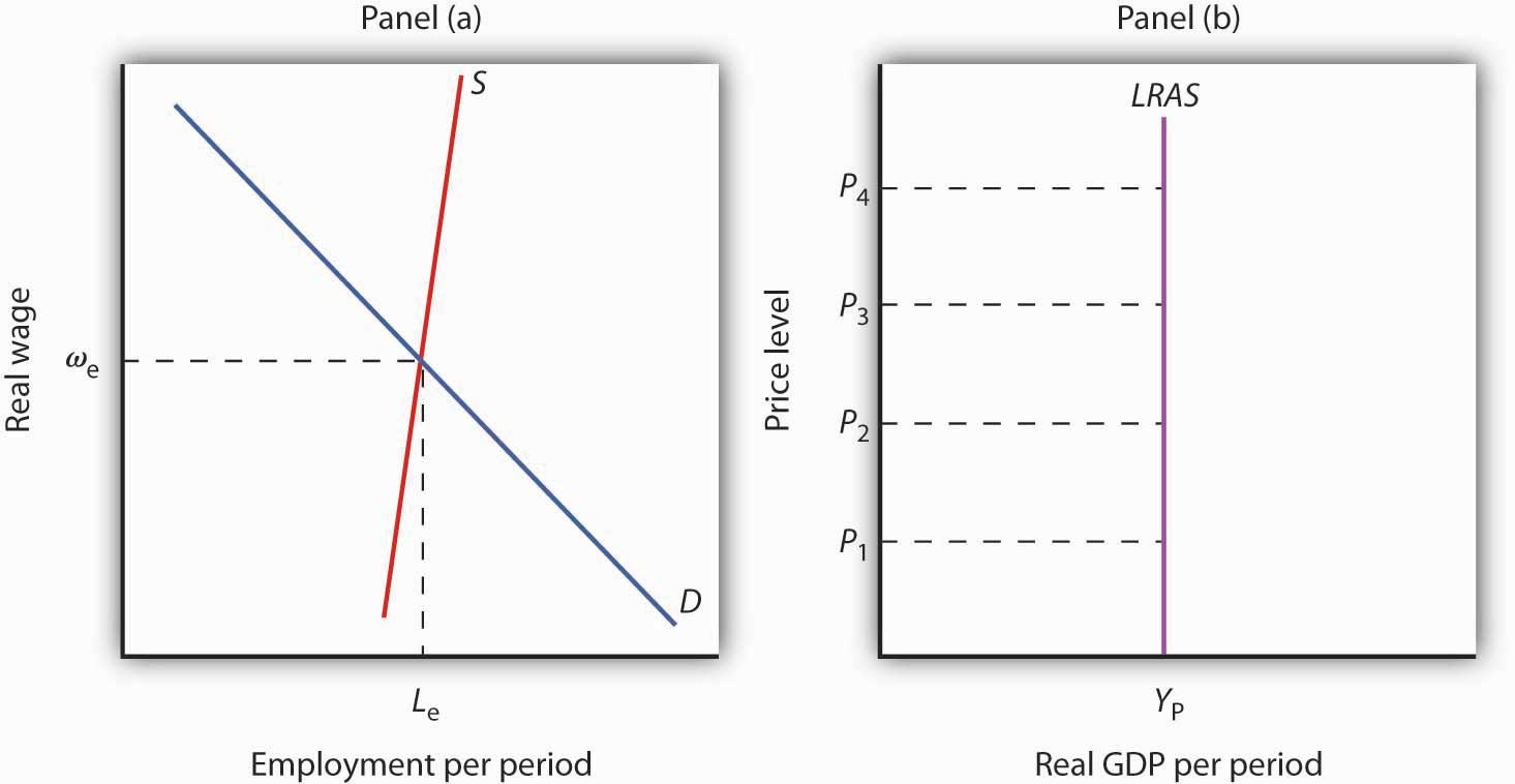
When the economy achieves its natural level of employment, as shown in Panel (a) at the intersection of the demand and supply curves for labor, it achieves its potential output, as shown in Panel (b) by the vertical long-run aggregate supply curve LRAS at YP.
In Panel (b) we see price levels ranging from P1 to P4. Higher price levels would require higher nominal wages to create a real wage of ωe, and flexible nominal wages would achieve that in the long run.
In the long run, then, the economy can achieve its natural level of employment and potential output at any price level. This conclusion gives us our long-run aggregate supply curve. With only one level of output at any price level, the long-run aggregate supply curve is a vertical line at the economy’s potential level of output of YP.
The intersection of the economy’s aggregate demand curve and the long-run aggregate supply curve determines its equilibrium real GDP and price level in the long run. Figure 7.5 "Long-Run Equilibrium" depicts an economy in long-run equilibrium. With aggregate demand at AD1 and the long-run aggregate supply curve as shown, real GDP is $12,000 billion per year and the price level is 1.14. If aggregate demand increases to AD2, long-run equilibrium will be reestablished at real GDP of $12,000 billion per year, but at a higher price level of 1.18. If aggregate demand decreases to AD3, long-run equilibrium will still be at real GDP of $12,000 billion per year, but with the now lower price level of 1.10.
Figure 7.5 Long-Run Equilibrium
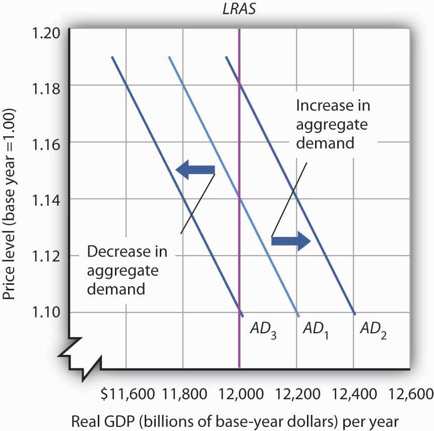
Long-run equilibrium occurs at the intersection of the aggregate demand curve and the long-run aggregate supply curve. For the three aggregate demand curves shown, long-run equilibrium occurs at three different price levels, but always at an output level of $12,000 billion per year, which corresponds to potential output.
Analysis of the macroeconomy in the short run—a period in which stickiness of wages and prices may prevent the economy from operating at potential output—helps explain how deviations of real GDP from potential output can and do occur. We will explore the effects of changes in aggregate demand and in short-run aggregate supply in this section.
Figure 7.6 Deriving the Short-Run Aggregate Supply Curve
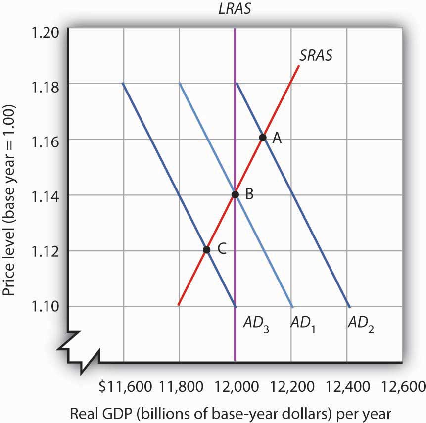
The economy shown here is in long-run equilibrium at the intersection of AD1 with the long-run aggregate supply curve. If aggregate demand increases to AD2, in the short run, both real GDP and the price level rise. If aggregate demand decreases to AD3, in the short run, both real GDP and the price level fall. A line drawn through points A, B, and C traces out the short-run aggregate supply curve SRAS.
The model of aggregate demand and long-run aggregate supply predicts that the economy will eventually move toward its potential output. To see how nominal wage and price stickiness can cause real GDP to be either above or below potential in the short run, consider the response of the economy to a change in aggregate demand. Figure 7.6 "Deriving the Short-Run Aggregate Supply Curve" shows an economy that has been operating at potential output of $12,000 billion and a price level of 1.14. This occurs at the intersection of AD1 with the long-run aggregate supply curve at point B. Now suppose that the aggregate demand curve shifts to the right (to AD2). This could occur as a result of an increase in exports. (The shift from AD1 to AD2 includes the multiplied effect of the increase in exports.) At the price level of 1.14, there is now excess demand and pressure on prices to rise. If all prices in the economy adjusted quickly, the economy would quickly settle at potential output of $12,000 billion, but at a higher price level (1.18 in this case).
Is it possible to expand output above potential? Yes. It may be the case, for example, that some people who were in the labor force but were frictionally or structurally unemployed find work because of the ease of getting jobs at the going nominal wage in such an environment. The result is an economy operating at point A in Figure 7.6 "Deriving the Short-Run Aggregate Supply Curve" at a higher price level and with output temporarily above potential.
Consider next the effect of a reduction in aggregate demand (to AD3), possibly due to a reduction in investment. As the price level starts to fall, output also falls. The economy finds itself at a price level–output combination at which real GDP is below potential, at point C. Again, price stickiness is to blame. The prices firms receive are falling with the reduction in demand. Without corresponding reductions in nominal wages, there will be an increase in the real wage. Firms will employ less labor and produce less output.
By examining what happens as aggregate demand shifts over a period when price adjustment is incomplete, we can trace out the short-run aggregate supply curve by drawing a line through points A, B, and C. The short-run aggregate supply (SRAS) curveA graphical representation of the relationship between production and the price level in the short run. is a graphical representation of the relationship between production and the price level in the short run. Among the factors held constant in drawing a short-run aggregate supply curve are the capital stock, the stock of natural resources, the level of technology, and the prices of factors of production.
A change in the price level produces a change in the aggregate quantity of goods and services suppliedMovement along the short-run aggregate supply curve. and is illustrated by the movement along the short-run aggregate supply curve. This occurs between points A, B, and C in Figure 7.6 "Deriving the Short-Run Aggregate Supply Curve".
A change in the quantity of goods and services supplied at every price level in the short run is a change in short-run aggregate supplyA change in the aggregate quantity of goods and services supplied at every price level in the short run.. Changes in the factors held constant in drawing the short-run aggregate supply curve shift the curve. (These factors may also shift the long-run aggregate supply curve; we will discuss them along with other determinants of long-run aggregate supply in the next chapter.)
One type of event that would shift the short-run aggregate supply curve is an increase in the price of a natural resource such as oil. An increase in the price of natural resources or any other factor of production, all other things unchanged, raises the cost of production and leads to a reduction in short-run aggregate supply. In Panel (a) of Figure 7.7 "Changes in Short-Run Aggregate Supply", SRAS1 shifts leftward to SRAS2. A decrease in the price of a natural resource would lower the cost of production and, other things unchanged, would allow greater production from the economy’s stock of resources and would shift the short-run aggregate supply curve to the right; such a shift is shown in Panel (b) by a shift from SRAS1 to SRAS3.
Figure 7.7 Changes in Short-Run Aggregate Supply
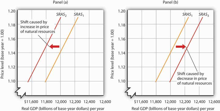
A reduction in short-run aggregate supply shifts the curve from SRAS1 to SRAS2 in Panel (a). An increase shifts it to the right to SRAS3, as shown in Panel (b).
Wage or price stickiness means that the economy may not always be operating at potential. Rather, the economy may operate either above or below potential output in the short run. Correspondingly, the overall unemployment rate will be below or above the natural level.
Many prices observed throughout the economy do adjust quickly to changes in market conditions so that equilibrium, once lost, is quickly regained. Prices for fresh food and shares of common stock are two such examples.
Other prices, though, adjust more slowly. Nominal wages, the price of labor, adjust very slowly. We will first look at why nominal wages are sticky, due to their association with the unemployment rate, a variable of great interest in macroeconomics, and then at other prices that may be sticky.
Wage contracts fix nominal wages for the life of the contract. The length of wage contracts varies from one week or one month for temporary employees, to one year (teachers and professors often have such contracts), to three years (for most union workers employed under major collective bargaining agreements). The existence of such explicit contracts means that both workers and firms accept some wage at the time of negotiating, even though economic conditions could change while the agreement is still in force.
Think about your own job or a job you once had. Chances are you go to work each day knowing what your wage will be. Your wage does not fluctuate from one day to the next with changes in demand or supply. You may have a formal contract with your employer that specifies what your wage will be over some period. Or you may have an informal understanding that sets your wage. Whatever the nature of your agreement, your wage is “stuck” over the period of the agreement. Your wage is an example of a sticky price.
One reason workers and firms may be willing to accept long-term nominal wage contracts is that negotiating a contract is a costly process. Both parties must keep themselves adequately informed about market conditions. Where unions are involved, wage negotiations raise the possibility of a labor strike, an eventuality that firms may prepare for by accumulating additional inventories, also a costly process. Even when unions are not involved, time and energy spent discussing wages takes away from time and energy spent producing goods and services. In addition, workers may simply prefer knowing that their nominal wage will be fixed for some period of time.
Some contracts do attempt to take into account changing economic conditions, such as inflation, through cost-of-living adjustments, but even these relatively simple contingencies are not as widespread as one might think. One reason might be that a firm is concerned that while the aggregate price level is rising, the prices for the goods and services it sells might not be moving at the same rate. Also, cost-of-living or other contingencies add complexity to contracts that both sides may want to avoid.
Even markets where workers are not employed under explicit contracts seem to behave as if such contracts existed. In these cases, wage stickiness may stem from a desire to avoid the same uncertainty and adjustment costs that explicit contracts avert.
Finally, minimum wage laws prevent wages from falling below a legal minimum, even if unemployment is rising. Unskilled workers are particularly vulnerable to shifts in aggregate demand.
Rigidity of other prices becomes easier to explain in light of the arguments about nominal wage stickiness. Since wages are a major component of the overall cost of doing business, wage stickiness may lead to output price stickiness. With nominal wages stable, at least some firms can adopt a “wait and see” attitude before adjusting their prices. During this time, they can evaluate information about why sales are rising or falling (Is the change in demand temporary or permanent?) and try to assess likely reactions by consumers or competing firms in the industry to any price changes they might make (Will consumers be angered by a price increase, for example? Will competing firms match price changes?).
In the meantime, firms may prefer to adjust output and employment in response to changing market conditions, leaving product price alone. Quantity adjustments have costs, but firms may assume that the associated risks are smaller than those associated with price adjustments.
Another possible explanation for price stickiness is the notion that there are adjustment costs associated with changing prices. In some cases, firms must print new price lists and catalogs, and notify customers of price changes. Doing this too often could jeopardize customer relations.
Yet another explanation of price stickiness is that firms may have explicit long-term contracts to sell their products to other firms at specified prices. For example, electric utilities often buy their inputs of coal or oil under long-term contracts.
Taken together, these reasons for wage and price stickiness explain why aggregate price adjustment may be incomplete in the sense that the change in the price level is insufficient to maintain real GDP at its potential level. These reasons do not lead to the conclusion that no price adjustments occur. But the adjustments require some time. During this time, the economy may remain above or below its potential level of output.
To illustrate how we will use the model of aggregate demand and aggregate supply, let us examine the impact of two events: an increase in the cost of health care and an increase in government purchases. The first reduces short-run aggregate supply; the second increases aggregate demand. Both events change equilibrium real GDP and the price level in the short run.
In the United States, most people receive health insurance for themselves and their families through their employers. In fact, it is quite common for employers to pay a large percentage of employees’ health insurance premiums, and this benefit is often written into labor contracts. As the cost of health care has gone up over time, firms have had to pay higher and higher health insurance premiums. With nominal wages fixed in the short run, an increase in health insurance premiums paid by firms raises the cost of employing each worker. It affects the cost of production in the same way that higher wages would. The result of higher health insurance premiums is that firms will choose to employ fewer workers.
Suppose the economy is operating initially at the short-run equilibrium at the intersection of AD1 and SRAS1, with a real GDP of Y1 and a price level of P1, as shown in Figure 7.8 "An Increase in Health Insurance Premiums Paid by Firms". This is the initial equilibrium price and output in the short run. The increase in labor cost shifts the short-run aggregate supply curve to SRAS2. The price level rises to P2 and real GDP falls to Y2.
Figure 7.8 An Increase in Health Insurance Premiums Paid by Firms
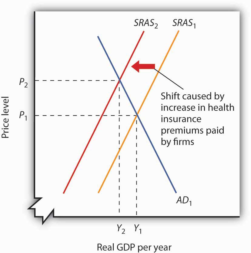
An increase in health insurance premiums paid by firms increases labor costs, reducing short-run aggregate supply from SRAS1 to SRAS2. The price level rises from P1 to P2 and output falls from Y1 to Y2.
A reduction in health insurance premiums would have the opposite effect. There would be a shift to the right in the short-run aggregate supply curve with pressure on the price level to fall and real GDP to rise.
Suppose the federal government increases its spending for highway construction. This circumstance leads to an increase in U.S. government purchases and an increase in aggregate demand.
Assuming no other changes affect aggregate demand, the increase in government purchases shifts the aggregate demand curve by a multiplied amount of the initial increase in government purchases to AD2 in Figure 7.9 "An Increase in Government Purchases". Real GDP rises from Y1 to Y2, while the price level rises from P1 to P2. Notice that the increase in real GDP is less than it would have been if the price level had not risen.
Figure 7.9 An Increase in Government Purchases
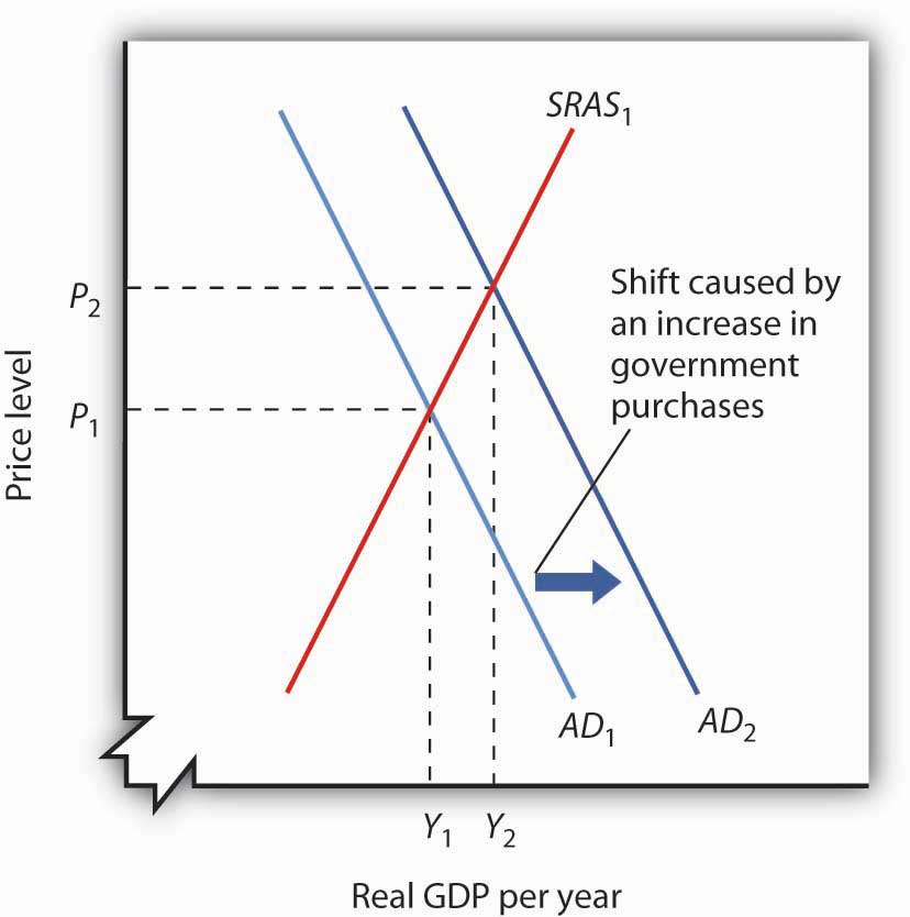
An increase in government purchases boosts aggregate demand from AD1 to AD2. Short-run equilibrium is at the intersection of AD2 and the short-run aggregate supply curve SRAS1. The price level rises to P2 and real GDP rises to Y2.
In contrast, a reduction in government purchases would reduce aggregate demand. The aggregate demand curve shifts to the left, putting pressure on both the price level and real GDP to fall.
In the short run, real GDP and the price level are determined by the intersection of the aggregate demand and short-run aggregate supply curves. Recall, however, that the short run is a period in which sticky prices may prevent the economy from reaching its natural level of employment and potential output. In the next section, we will see how the model adjusts to move the economy to long-run equilibrium and what, if anything, can be done to steer the economy toward the natural level of employment and potential output.
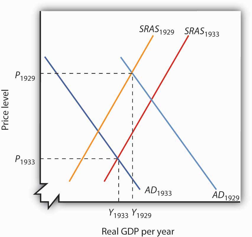
The tools we have covered in this section can be used to understand the Great Depression of the 1930s. We know that investment and consumption began falling in late 1929. The reductions were reinforced by plunges in net exports and government purchases over the next four years. In addition, nominal wages plunged 26% between 1929 and 1933. We also know that real GDP in 1933 was 30% below real GDP in 1929. Use the tools of aggregate demand and short-run aggregate supply to graph and explain what happened to the economy between 1929 and 1933.
What were the causes of the U.S. recession of 2001? Economist Kevin Kliesen of the Federal Reserve Bank of St. Louis points to four factors that, taken together, shifted the aggregate demand curve to the left and kept it there for a long enough period to keep real GDP falling for about nine months. They were the fall in stock market prices, the decrease in business investment both for computers and software and in structures, the decline in the real value of exports, and the aftermath of 9/11. Notable exceptions to this list of culprits were the behavior of consumer spending during the period and new residential housing, which falls into the investment category.
During the expansion in the late 1990s, a surging stock market probably made it easier for firms to raise funding for investment in both structures and information technology. Even though the stock market bubble burst well before the actual recession, the continuation of projects already underway delayed the decline in the investment component of GDP. Also, spending for information technology was probably prolonged as firms dealt with Y2K computing issues, that is, computer problems associated with the change in the date from 1999 to 2000. Most computers used only two digits to indicate the year, and when the year changed from ’99 to ’00, computers did not know how to interpret the change, and extensive reprogramming of computers was required.
Real exports fell during the recession because (1) the dollar was strong during the period and (2) real GDP growth in the rest of the world fell almost 5% from 2000 to 2001.
Then, the terrorist attacks of 9/11, which literally shut down transportation and financial markets for several days, may have prolonged these negative tendencies just long enough to turn what might otherwise have been a mild decline into enough of a downtown to qualify the period as a recession.
During this period the measured price level was essentially stable—with the implicit price deflator rising by less than 1%. Thus, while the aggregate demand curve shifted left as a result of all the reasons given above, there was also a leftward shift in the short-run aggregate supply curve.
Source: Kevin L. Kliesen, “The 2001 Recession: How Was It Different and What Developments May Have Caused It?,” The Federal Reserve Bank of St. Louis Review, September/October 2003, 23–37.
All components of aggregate demand (consumption, investment, government purchases, and net exports) declined between 1929 and 1933. Thus the aggregate demand curve shifted markedly to the left, moving from AD1929 to AD1933. The reduction in nominal wages corresponds to an increase in short-run aggregate supply from SRAS1929 to SRAS1933. Since real GDP in 1933 was less than real GDP in 1929, we know that the movement in the aggregate demand curve was greater than that of the short-run aggregate supply curve.