Fiscal policy—the use of government expenditures and taxes to influence the level of economic activity—is the government counterpart to monetary policy. Like monetary policy, it can be used in an effort to close a recessionary or an inflationary gap.
Some tax and expenditure programs change automatically with the level of economic activity. We will examine these first. Then we will look at how discretionary fiscal policies work. Four examples of discretionary fiscal policy choices were the tax cuts introduced by the Kennedy, Reagan, and George W. Bush administrations and the increase in government purchases proposed by President Clinton in 1993. The 2009 fiscal stimulus bill passed in the first months of the administration of Barack Obama included both tax rebates and spending increases. All were designed to stimulate aggregate demand and close recessionary gaps.
Certain government expenditure and taxation policies tend to insulate individuals from the impact of shocks to the economy. Transfer payments have this effect. Because more people become eligible for income supplements when income is falling, transfer payments reduce the effect of a change in real GDP on disposable personal income and thus help to insulate households from the impact of the change. Income taxes also have this effect. As incomes fall, people pay less in income taxes.
Any government program that tends to reduce fluctuations in GDP automatically is called an automatic stabilizerAny government program that tends to reduce fluctuations in GDP automatically.. Automatic stabilizers tend to increase GDP when it is falling and reduce GDP when it is rising.
To see how automatic stabilizers work, consider the decline in real GDP that occurred during the recession of 1990–1991. Real GDP fell 1.6% from the peak to the trough of that recession. The reduction in economic activity automatically reduced tax payments, reducing the impact of the downturn on disposable personal income. Furthermore, the reduction in incomes increased transfer payment spending, boosting disposable personal income further. Real disposable personal income thus fell by only 0.9% during the 1990—1991 recession, a much smaller percentage than the reduction in real GDP. Rising transfer payments and falling tax collections helped cushion households from the impact of the recession and kept real GDP from falling as much as it would have otherwise.
Automatic stabilizers have emerged as key elements of fiscal policy. Increases in income tax rates and unemployment benefits have enhanced their importance as automatic stabilizers. The introduction in the 1960s and 1970s of means-tested federal transfer payments, in which individuals qualify depending on their income, added to the nation’s arsenal of automatic stabilizers. The advantage of automatic stabilizers is suggested by their name. As soon as income starts to change, they go to work. Because they affect disposable personal income directly, and because changes in disposable personal income are closely linked to changes in consumption, automatic stabilizers act swiftly to reduce the degree of changes in real GDP.
It is important to note that changes in expenditures and taxes that occur through automatic stabilizers do not shift the aggregate demand curve. Because they are automatic, their operation is already incorporated in the curve itself.
As we begin to look at deliberate government efforts to stabilize the economy through fiscal policy choices, we note that most of the government’s taxing and spending is for purposes other than economic stabilization. For example, the increase in defense spending in the early 1980s under President Ronald Reagan and in the administration of George W. Bush were undertaken primarily to promote national security. That the increased spending affected real GDP and employment was a by-product. The effect of such changes on real GDP and the price level is secondary, but it cannot be ignored. Our focus here, however, is on discretionary fiscal policy that is undertaken with the intention of stabilizing the economy. As we have seen, the tax cuts introduced by the Bush administration were justified as expansionary measures.
Discretionary government spending and tax policies can be used to shift aggregate demand. Expansionary fiscal policy might consist of an increase in government purchases or transfer payments, a reduction in taxes, or a combination of these tools to shift the aggregate demand curve to the right. A contractionary fiscal policy might involve a reduction in government purchases or transfer payments, an increase in taxes, or a mix of all three to shift the aggregate demand curve to the left.
Figure 12.8 "Expansionary and Contractionary Fiscal Policies to Shift Aggregate Demand" illustrates the use of fiscal policy to shift aggregate demand in response to a recessionary gap and an inflationary gap. In Panel (a), the economy produces a real GDP of Y1, which is below its potential level of Yp. An expansionary fiscal policy seeks to shift aggregate demand to AD2 in order to close the gap. In Panel (b), the economy initially has an inflationary gap at Y1. A contractionary fiscal policy seeks to reduce aggregate demand to AD2 and close the gap. Now we shall look at how specific fiscal policy options work. In our preliminary analysis of the effects of fiscal policy on the economy, we will assume that at a given price level these policies do not affect interest rates or exchange rates. We will relax that assumption later in the chapter.
Figure 12.8 Expansionary and Contractionary Fiscal Policies to Shift Aggregate Demand
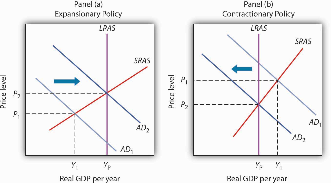
In Panel (a), the economy faces a recessionary gap (YP − Y1). An expansionary fiscal policy seeks to shift aggregate demand to AD2 to close the gap. In Panel (b), the economy faces an inflationary gap (Y1 − YP). A contractionary fiscal policy seeks to reduce aggregate demand to AD2 to close the gap.
One policy through which the government could seek to shift the aggregate demand curve is a change in government purchases. We learned that the aggregate demand curve shifts to the right by an amount equal to the initial change in government purchases times the multiplier. This multiplied effect of a change in government purchases occurs because the increase in government purchases increases income, which in turn increases consumption. Then, part of the impact of the increase in aggregate demand is absorbed by higher prices, preventing the full increase in real GDP that would have occurred if the price level did not rise.
Figure 12.9 "An Increase in Government Purchases" shows the effect of an increase in government purchases of $200 billion. The initial price level is P1 and the initial equilibrium real GDP is $12,000 billion. Suppose the multiplier is 2. The $200 billion increase in government purchases increases the total quantity of goods and services demanded, at a price level of P1, by $400 billion (the $200 billion increase in government purchases times the multiplier) to $12,400 billion. The aggregate demand thus shifts to the right by that amount to AD2. The equilibrium level of real GDP rises to $12,300 billion, and the price level rises to P2.
Figure 12.9 An Increase in Government Purchases
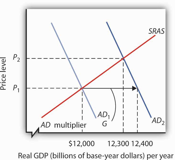
The economy shown here is initially in equilibrium at a real GDP of $12,000 billion and a price level of P1. An increase of $200 billion in the level of government purchases (ΔG) shifts the aggregate demand curve to the right by $400 billion to AD2. The equilibrium level of real GDP rises to $12,300 billion, while the price level rises to P2.
A reduction in government purchases would have the opposite effect. The aggregate demand curve would shift to the left by an amount equal to the initial change in government purchases times the multiplier. Real GDP and the price level would fall.
One of the first fiscal policy measures undertaken by the Kennedy administration in the 1960s was an investment tax credit. An investment tax credit allows a firm to reduce its tax liability by a percentage of the investment it undertakes during a particular period. With an investment tax credit of 10%, for example, a firm that engaged in $1 million worth of investment during a year could reduce its tax liability for that year by $100,000. The investment tax credit introduced by the Kennedy administration was later repealed. It was reintroduced during the Reagan administration in 1981, then abolished by the Tax Reform Act of 1986. President Clinton called for a new investment tax credit in 1993 as part of his job stimulus proposal, but that proposal was rejected by Congress. The Bush administration reinstated the investment tax credit as part of its tax cut package.
An investment tax credit is intended, of course, to stimulate additional private sector investment. A reduction in the tax rate on corporate profits would be likely to have a similar effect. Conversely, an increase in the corporate income tax rate or a reduction in an investment tax credit could be expected to reduce investment.
A change in investment affects the aggregate demand curve in precisely the same manner as a change in government purchases. It shifts the aggregate demand curve by an amount equal to the initial change in investment times the multiplier.
An increase in the investment tax credit, or a reduction in corporate income tax rates, will increase investment and shift the aggregate demand curve to the right. Real GDP and the price level will rise. A reduction in the investment tax credit, or an increase in corporate income tax rates, will reduce investment and shift the aggregate demand curve to the left. Real GDP and the price level will fall.Investment also affects the long-run aggregate supply curve, since a change in the capital stock changes the potential level of real GDP. We examined this earlier in the chapter on economic growth.
Income taxes affect the consumption component of aggregate demand. An increase in income taxes reduces disposable personal income and thus reduces consumption (but by less than the change in disposable personal income). That shifts the aggregate demand curve leftward by an amount equal to the initial change in consumption that the change in income taxes produces times the multiplier.A change in tax rates will change the value of the multiplier. The reason is explained in another chapter. A reduction in income taxes increases disposable personal income, increases consumption (but by less than the change in disposable personal income), and increases aggregate demand.
Suppose, for example, that income taxes are reduced by $200 billion. Only some of the increase in disposable personal income will be used for consumption and the rest will be saved. Suppose the initial increase in consumption is $180 billion. Then the shift in the aggregate demand curve will be a multiple of $180 billion; if the multiplier is 2, aggregate demand will shift to the right by $360 billion. Thus, as compared to the $200-billion increase in government purchases that we saw in Figure 12.9 "An Increase in Government Purchases", the shift in the aggregate demand curve due to an income tax cut is somewhat less, as is the effect on real GDP and the price level.
Changes in transfer payments, like changes in income taxes, alter the disposable personal income of households and thus affect their consumption, which is a component of aggregate demand. A change in transfer payments will thus shift the aggregate demand curve because it will affect consumption. Because consumption will change by less than the change in disposable personal income, a change in transfer payments of some amount will result in a smaller change in real GDP than would a change in government purchases of the same amount. As with income taxes, a $200-billion increase in transfer payments will shift the aggregate demand curve to the right by less than the $200-billion increase in government purchases that we saw in Figure 12.9 "An Increase in Government Purchases".
Table 12.1 "Fiscal Policy in the United States Since 1964" summarizes U.S. fiscal policies undertaken to shift aggregate demand since the 1964 tax cuts. We see that expansionary policies have been chosen in response to recessionary gaps and that contractionary policies have been chosen in response to inflationary gaps. Changes in government purchases and in taxes have been the primary tools of fiscal policy in the United States.
Table 12.1 Fiscal Policy in the United States Since 1964
| Year | Situation | Policy response |
|---|---|---|
| 1968 | Inflationary gap | A temporary tax increase, first recommended by President Johnson’s Council of Economic Advisers in 1965, goes into effect. This one-time surcharge of 10% is added to individual income tax liabilities. |
| 1969 | Inflationary gap | President Nixon, facing a continued inflationary gap, orders cuts in government purchases. |
| 1975 | Recessionary gap | President Ford, facing a recession induced by an OPEC oil-price increase, proposes a temporary 10% tax cut. It is passed almost immediately and goes into effect within two months. |
| 1981 | Recessionary gap | President Reagan had campaigned on a platform of increased defense spending and a sharp cut in income taxes. The tax cuts are approved in 1981 and are implemented over a period of three years. The increased defense spending begins in 1981. While the Reagan administration rejects the use of fiscal policy as a stabilization tool, its policies tend to increase aggregate demand early in the 1980s. |
| 1992 | Recessionary gap | President Bush had rejected the use of expansionary fiscal policy during the recession of 1990–1991. Indeed, he agreed late in 1990 to a cut in government purchases and a tax increase. In a campaign year, however, he orders a cut in withholding rates designed to increase disposable personal income in 1992 and to boost consumption. |
| 1993 | Recessionary gap | President Clinton calls for a $16-billion jobs package consisting of increased government purchases and tax cuts aimed at stimulating investment. The president says the plan will create 500,000 new jobs. The measure is rejected by Congress. |
| 2001 | Recessionary gap | President Bush campaigned to reduce taxes in order to reduce the size of government and encourage long-term growth. When he took office in 2001, the economy was weak and the $1.35-billion tax cut was aimed at both long-term tax relief and at stimulating the economy in the short term. It included, for example, a personal income tax rebate of $300 to $600 per household. With unemployment still high a couple of years into the expansion, another tax cut was passed in 2003. |
| 2008 | Recessionary gap | Fiscal stimulus package of $150 billion to spur economy. It included $100 billion in tax rebates and $50 billion in tax cuts for businesses. |
| 2009 | Recessionary gap | Fiscal stimulus package of $784 billion included tax rebates and increased government spending passed in early days of President Obama’s administration. |
| 2010–2012 | Recessionary gap | Extensions of the payroll tax reduction and unemployment insurance benefits continued. |
Suppose the economy has an inflationary gap. What fiscal policies might be used to close the gap? Using the model of aggregate demand and aggregate supply, illustrate the effect of these policies.

There is a wide range of opinions among economists regarding the size of the fiscal multiplier. In 2011, the American Economic Association’s Journal of Economic Literature published three papers on this topic in a special section titled “Forum: The Multiplier.” The papers provide at least two-and-a-half different answers!
In her paper titled “Can Government Purchases Stimulate the Economy?,” Valerie Ramey concludes that the size of the government purchases multiplier depends on many factors but that, when the increase in government purchases is temporary and financed by government borrowing, the multiplier “is probably between 0.8 and 1.5. Reasonable people can argue, however, that the data do not reject 0.5 to 2.” This is quite a wide range.
In “An Empirical Analysis of the Revival of Fiscal Activism in the 2000s,” John Taylor argues that the various components of the recent fiscal packages (tax cuts, aid to states, and increased government purchases) had little effect on the economy—implying a multiplier of zero or nearly so. Using aggregate quarterly data simulations for the 2000s, he argues that transfers and tax cuts were used by households to increase saving, that the increase in government purchases were too small to have made much of a difference, and that state and local governments used their stimulus dollars for transfers or to reduce their borrowing.
In “On Measuring the Effects of Fiscal Policy in Recessions,” Jonathan Parker essentially argues that the statistical models built to date are ultimately inadequate and that we will only be able to get at the answer as better and more refined studies are conducted. Noting that the multiplier effect of fiscal policy is likely to depend on the state of the economy, he concludes that “an important difficulty with further investigation is the limited macroeconomic data available on the effects of policy in recessions (or deep recessions).” Perhaps we need a few more Great Recessions in order to figure this out.
In another American Economic Association publication, the Journal of Economic Perspectives, Alan Auerbach, William Gale, and Benjamin Harris provide an extensive review of the variety in multiplier estimates, which they acknowledge is “embarrassingly large” after so many years of trying to measure it. Concerning the 2009 American Recovery and Reinvestment Act, though, they write, “If a fiscal stimulus were ever to be considered appropriate, the beginning of 2009 was such a time.…In these circumstances, our judgment is that a fiscal expansion carried much smaller risks than the lack of one would have.”
Sources: Alan J. Auerbach, William G. Gale, and Benjamin H. Harris, “Activist Fiscal Policy,” Journal of Economic Perspectives 24, no. 4 (Fall 2010): 141–64; Jonathan A. Parker, “On Measuring the Effects of Fiscal Policy in Recessions,” Journal of Economic Literature 49, no. 3 (September 2011): 703–18; Valerie A. Ramey, “Can Government Purchases Stimulate the Economy?,” Journal of Economic Literature 49, no. 3 (September 2011): 673–85; John B. Taylor, “An Empirical Analysis of the Revival of Fiscal Activism in the 2000s,” Journal of Economic Literature 49, no. 3 (September 2011): 686–702.
Fiscal policies that could be used to close an inflationary gap include reductions in government purchases and transfer payments and increases in taxes. As shown in Panel (b) of Figure 12.8 "Expansionary and Contractionary Fiscal Policies to Shift Aggregate Demand", the goal would be to shift the aggregate demand curve to the left so that it will intersect the short-run aggregate supply curve at YP.


