2008 turned out to be the worst holiday shopping season in decades. Why? U.S. consumers were battered from many directions. Housing prices had fallen nearly 20% over the year. The stock market had fallen over 40%. Interest rates were falling, but credit was extremely hard to come by. By December, consumer confidence hit an all-time low amid concerns of rising unemployment. Cutting back seemed like the best defense for weathering this tough environment.
Consumption accounts for the bulk of aggregate demand in the United States and in other countries. In this chapter, we will examine the determinants of consumption and introduce a new model, the aggregate expenditures model, which will give insights into the aggregate demand curve. Any change in aggregate demand causes a change in income, and a change in income causes a change in consumption—which changes aggregate demand and thus income and thus consumption. The aggregate expenditures model will help us to unravel the important relationship between consumption and real GDP.
J. R. McCulloch, an economist of the early nineteenth century, wrote, “Consumption … is, in fact, the object of industry.”J. R. Mc Culloch, A Discourse on the Rise, Progress, Peculiar Objects, and Importance, of Political Economy: Containing the Outline of a Course of Lectures on the Principles and Doctrines of That Science (Edinburgh: Archibald Constable, 1824), 103. Goods and services are produced so that people can use them. The factors that determine consumption thus determine how successful an economy is in fulfilling its ultimate purpose: providing goods and services for people. So, consumption is not just important because it is such a large component of economic activity. It is important because, as McCulloch said, consumption is at the heart of the economy’s fundamental purpose.
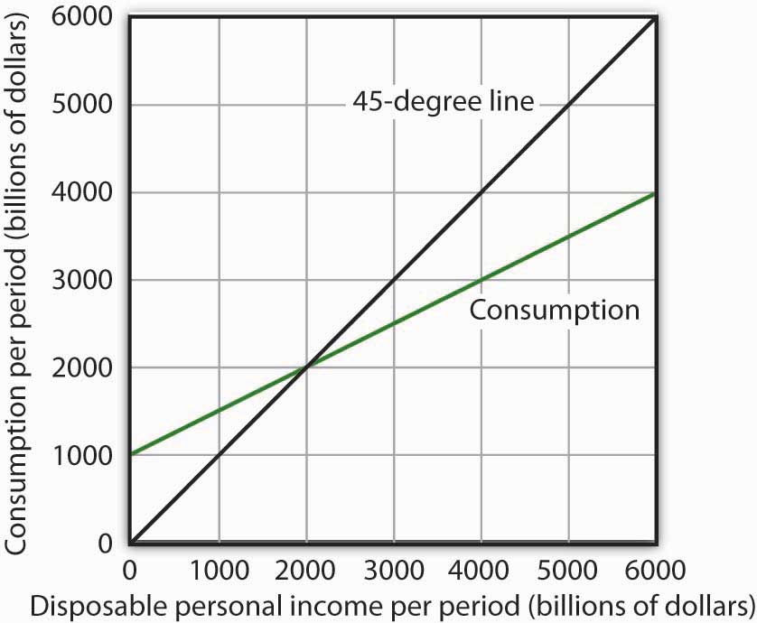
It seems reasonable to expect that consumption spending by households will be closely related to their disposable personal income, which equals the income households receive less the taxes they pay. Note that disposable personal income and GDP are not the same thing. GDP is a measure of total income; disposable personal income is the income households have available to spend during a specified period.
Real values of disposable personal income and consumption per year from 1960 through 2011 are plotted in Figure 13.1 "The Relationship between Consumption and Disposable Personal Income, 1960–2011". The data suggest that consumption generally changes in the same direction as does disposable personal income.
The relationship between consumption and disposable personal income is called the consumption functionThe relationship between consumption and disposable personal income.. It can be represented algebraically as an equation, as a schedule in a table, or as a curve on a graph.
Figure 13.1 The Relationship between Consumption and Disposable Personal Income, 1960–2011
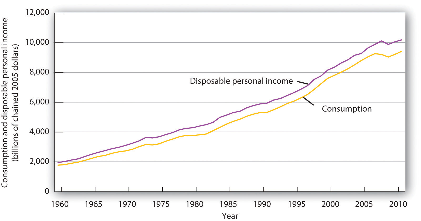
Plots of consumption and disposable personal income over time suggest that consumption increases as disposable personal income increases.
Source: U. S. Department of Commerce, Bureau of Economic Analysis, NIPA Tables 1.1.6 and 2.1 (revised February 29, 2012).
Figure 13.2 "Plotting a Consumption Function" illustrates the consumption function. The relationship between consumption and disposable personal income that we encountered in Figure 13.1 "The Relationship between Consumption and Disposable Personal Income, 1960–2011" is evident in the table and in the curve: consumption in any period increases as disposable personal income increases in that period. The slope of the consumption function tells us by how much. Consider points C and D. When disposable personal income (Yd) rises by $500 billion, consumption rises by $400 billion. More generally, the slope equals the change in consumption divided by the change in disposable personal income. The ratio of the change in consumption (ΔC) to the change in disposable personal income (ΔYd) is the marginal propensity to consumeThe ratio of the change in consumption (ΔC) to the change in disposable personal income (ΔYd). (MPC). The Greek letter delta (Δ) is used to denote “change in.”
Equation 13.1
In this case, the marginal propensity to consume equals $400/$500 = 0.8. It can be interpreted as the fraction of an extra $1 of disposable personal income that people spend on consumption. Thus, if a person with an MPC of 0.8 received an extra $1,000 of disposable personal income, that person’s consumption would rise by $0.80 for each extra $1 of disposable personal income, or $800.
We can also express the consumption function as an equation
Equation 13.2
Figure 13.2 Plotting a Consumption Function
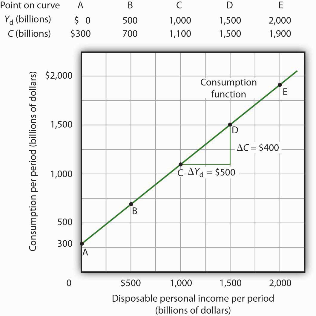
The consumption function relates consumption C to disposable personal income Yd. The equation for the consumption function shown here in tabular and graphical form is C = $300 billion + 0.8Yd.
It is important to note carefully the definition of the marginal propensity to consume. It is the change in consumption divided by the change in disposable personal income. It is not the level of consumption divided by the level of disposable personal income. Using Equation 13.2, at a level of disposable personal income of $500 billion, for example, the level of consumption will be $700 billion so that the ratio of consumption to disposable personal income will be 1.4, while the marginal propensity to consume remains 0.8. The marginal propensity to consume is, as its name implies, a marginal concept. It tells us what will happen to an additional dollar of personal disposable income.
Notice from the curve in Figure 13.2 "Plotting a Consumption Function" that when disposable personal income equals 0, consumption is $300 billion. The vertical intercept of the consumption function is thus $300 billion. Then, for every $500 billion increase in disposable personal income, consumption rises by $400 billion. Because the consumption function in our example is linear, its slope is the same between any two points. In this case, the slope of the consumption function, which is the same as the marginal propensity to consume, is 0.8 all along its length.
We can use the consumption function to show the relationship between personal saving and disposable personal income. Personal savingDisposable personal income not spent on consumption during a particular period. is disposable personal income not spent on consumption during a particular period; the value of personal saving for any period is found by subtracting consumption from disposable personal income for that period:
Equation 13.3
The saving functionThe relationship between personal saving in any period and disposable personal income in that period. relates personal saving in any period to disposable personal income in that period. Personal saving is not the only form of saving—firms and government agencies may save as well. In this chapter, however, our focus is on the choice households make between using disposable personal income for consumption or for personal saving.
Figure 13.3 "Consumption and Personal Saving" shows how the consumption function and the saving function are related. Personal saving is calculated by subtracting values for consumption from values for disposable personal income, as shown in the table. The values for personal saving are then plotted in the graph. Notice that a 45-degree line has been added to the graph. At every point on the 45-degree line, the value on the vertical axis equals that on the horizontal axis. The consumption function intersects the 45-degree line at an income of $1,500 billion (point D). At this point, consumption equals disposable personal income and personal saving equals 0 (point D′ on the graph of personal saving). Using the graph to find personal saving at other levels of disposable personal income, we subtract the value of consumption, given by the consumption function, from disposable personal income, given by the 45-degree line.
Figure 13.3 Consumption and Personal Saving
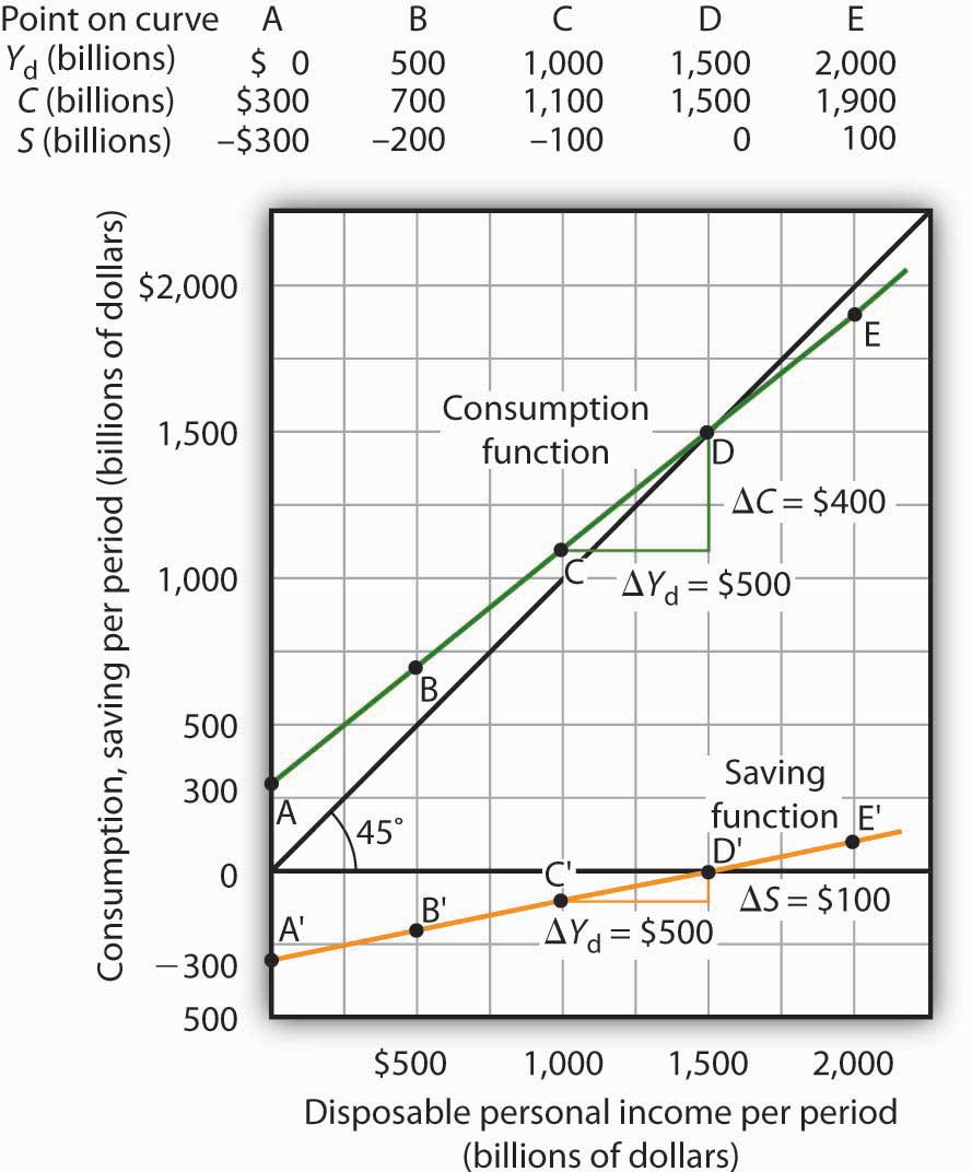
Personal saving equals disposable personal income minus consumption. The table gives hypothetical values for these variables. The consumption function is plotted in the upper part of the graph. At points along the 45-degree line, the values on the two axes are equal; we can measure personal saving as the distance between the 45-degree line and consumption. The curve of the saving function is in the lower portion of the graph.
At a disposable personal income of $2,000 billion, for example, consumption is $1,900 billion (point E). Personal saving equals $100 billion (point E′)—the vertical distance between the 45-degree line and the consumption function. At an income of $500 billion, consumption totals $700 billion (point B). The consumption function lies above the 45-degree line at this point; personal saving is −$200 billion (point B′). A negative value for saving means that consumption exceeds disposable personal income; it must have come from saving accumulated in the past, from selling assets, or from borrowing.
Notice that for every $500 billion increase in disposable personal income, personal saving rises by $100 billion. Consider points C′ and D′ in Figure 13.3 "Consumption and Personal Saving". When disposable personal income rises by $500 billion, personal saving rises by $100 billion. More generally, the slope of the saving function equals the change in personal saving divided by the change in disposable personal income. The ratio of the change in personal saving (ΔS) to the change in disposable personal income (ΔYd) is the marginal propensity to saveThe ratio of the change in personal saving (ΔS) to the change in disposable personal income (ΔYd). (MPS).
Equation 13.4
In this case, the marginal propensity to save equals $100/$500 = 0.2. It can be interpreted as the fraction of an extra $1 of disposable personal income that people save. Thus, if a person with an MPS of 0.2 received an extra $1,000 of disposable personal income, that person’s saving would rise by $0.20 for each extra $1 of disposable personal income, or $200. Since people have only two choices of what to do with additional disposable personal income—that is, they can use it either for consumption or for personal saving—the fraction of disposable personal income that people consume (MPC) plus the fraction of disposable personal income that people save (MPS) must add to 1:
Equation 13.5
The discussion so far has related consumption in a particular period to income in that same period. The current income hypothesisConsumption in any one period depends on income during that period. holds that consumption in any one period depends on income during that period, or current income.
Although it seems obvious that consumption should be related to disposable personal income, it is not so obvious that consumers base their consumption in any one period on the income they receive during that period. In buying a new car, for example, consumers might base their decision not only on their current income but on the income they expect to receive during the three or four years they expect to be making payments on the car. Parents who purchase a college education for their children might base their decision on their own expected lifetime income.
Indeed, it seems likely that virtually all consumption choices could be affected by expectations of income over a very long period. One reason people save is to provide funds to live on during their retirement years. Another is to build an estate they can leave to their heirs through bequests. The amount people save for their retirement or for bequests depends on the income they expect to receive for the rest of their lives. For these and other reasons, then, personal saving (and thus consumption) in any one year is influenced by permanent income. Permanent incomeThe average annual income people expect to receive for the rest of their lives. is the average annual income people expect to receive for the rest of their lives.
People who have the same current income but different permanent incomes might reach very different saving decisions. Someone with a relatively low current income but a high permanent income (a college student planning to go to medical school, for example) might save little or nothing now, expecting to save for retirement and for bequests later. A person with the same low income but no expectation of higher income later might try to save some money now to provide for retirement or bequests later. Because a decision to save a certain amount determines how much will be available for consumption, consumption decisions can also be affected by expected lifetime income. Thus, an alternative approach to explaining consumption behavior is the permanent income hypothesisConsumption in any period depends on permanent income., which assumes that consumption in any period depends on permanent income. An important implication of the permanent income hypothesis is that a change in income regarded as temporary will not affect consumption much, since it will have little effect on average lifetime income; a change regarded as permanent will have an effect. The current income hypothesis, though, predicts that it does not matter whether consumers view a change in disposable personal income as permanent or temporary; they will move along the consumption function and change consumption accordingly.
The question of whether permanent or current income is a determinant of consumption arose in 1992 when President George H. W. Bush ordered a change in the withholding rate for personal income taxes. Workers have a fraction of their paychecks withheld for taxes each pay period; Mr. Bush directed that this fraction be reduced in 1992. The change in the withholding rate did not change income tax rates; by withholding less in 1992, taxpayers would either receive smaller refund checks in 1993 or owe more taxes. The change thus left taxpayers’ permanent income unaffected.
President Bush’s measure was designed to increase aggregate demand and close the recessionary gap created by the 1990–1991 recession. Economists who subscribed to the permanent income hypothesis predicted that the change would not have any effect on consumption. Those who subscribed to the current income hypothesis predicted that the measure would boost consumption substantially in 1992. A survey of households taken during this period suggested that households planned to spend about 43% of the temporary increase in disposable personal income produced by the withholding experiment.Matthew D. Shapiro and Joel Slemrod, “Consumer Response to the Timing of Income: Evidence from a Change in Tax Withholding,” American Economic Review 85 (March 1995): 274–83. That is considerably less than would be predicted by the current income hypothesis, but more than the zero change predicted by the permanent income hypothesis. This result, together with related evidence, suggests that temporary changes in income can affect consumption, but that changes regarded as permanent will have a much stronger impact.
Many of the tax cuts passed during the administration of President George W. Bush are set to expire at the end of 2012. The proposal to make these tax cuts permanent is aimed toward having a stronger impact on consumption, since tax cuts regarded as permanent have larger effects than do changes regarded as temporary.
The consumption function graphed in Figure 13.2 "Plotting a Consumption Function" and Figure 13.3 "Consumption and Personal Saving" relates consumption spending to the level of disposable personal income. Changes in disposable personal income cause movements along this curve; they do not shift the curve. The curve shifts when other determinants of consumption change. Examples of changes that could shift the consumption function are changes in real wealth and changes in expectations. Figure 13.4 "Shifts in the Consumption Function" illustrates how these changes can cause shifts in the curve.
Figure 13.4 Shifts in the Consumption Function
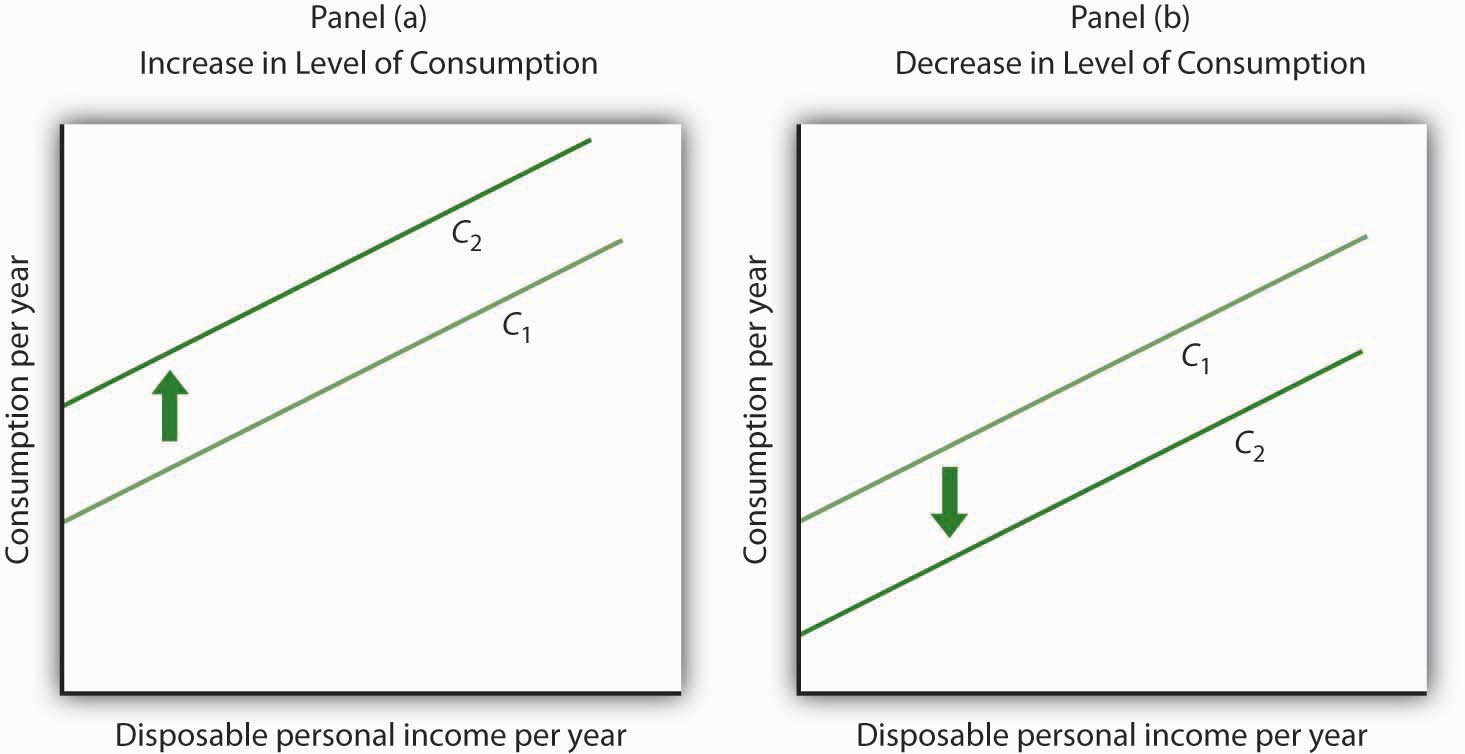
An increase in the level of consumption at each level of disposable personal income shifts the consumption function upward in Panel (a). Among the events that would shift the curve upward are an increase in real wealth and an increase in consumer confidence. A reduction in the level of consumption at each level of disposable personal income shifts the curve downward in Panel (b). The events that could shift the curve downward include a reduction in real wealth and a decline in consumer confidence.
An increase in stock and bond prices, for example, would make holders of these assets wealthier, and they would be likely to increase their consumption. An increase in real wealth shifts the consumption function upward, as illustrated in Panel (a) of Figure 13.4 "Shifts in the Consumption Function". A reduction in real wealth shifts it downward, as shown in Panel (b).
A change in the price level changes real wealth. We learned in an earlier chapter that the relationship among the price level, real wealth, and consumption is called the wealth effect. A reduction in the price level increases real wealth and shifts the consumption function upward, as shown in Panel (a). An increase in the price level shifts the curve downward, as shown in Panel (b).
Consumers are likely to be more willing to spend money when they are optimistic about the future. Surveyors attempt to gauge this optimism using “consumer confidence” surveys that ask respondents to report whether they are optimistic or pessimistic about their own economic situation and about the prospects for the economy as a whole. An increase in consumer optimism tends to shift the consumption function upward as in Panel (a) of Figure 13.4 "Shifts in the Consumption Function"; an increase in pessimism tends to shift it downward as in Panel (b). The sharp reduction in consumer confidence in 2008 and early in 2009 contributed to a downward shift in the consumption function and thus to the severity of the recession.
The relationship between consumption and consumer expectations concerning future economic conditions tends to be a form of self-fulfilling prophecy. If consumers expect economic conditions to worsen, they will cut their consumption—and economic conditions will worsen! Political leaders often try to persuade people that economic prospects are good. In part, such efforts are an attempt to increase economic activity by boosting consumption.
For each of the following events, draw a curve representing the consumption function and show how the event would affect the curve.

The first round of the Bush tax cuts was passed in 2001. Democrats in Congress insisted on a rebate aimed at stimulating consumption. In the summer of 2001, rebates of $300 per single taxpayer and of $600 for married couples were distributed. The Department of Treasury reported that 92 million people received the rebates. While the rebates were intended to stimulate consumption, the extent to which the tax rebates stimulated consumption, especially during the recession, is an empirical question.
It is difficult to analyze the impact of a tax rebate that is a single event experienced by all households at the same time. If spending does change at that moment, is it because of the tax rebate or because of some other event that occurred at that time?
Fortunately for researchers Sumit Agarwal, Chunlin Liu, and Nicholas Souleles, using data from credit card accounts, the 2001 tax rebate checks were distributed over 10 successive weeks from July to September of 2001. The timing of receipt was random, since it was based on the next-to-last digit of one’s Social Security number, and taxpayers were informed well in advance that the checks were coming. The researchers found that consumers initially saved much of their rebates, by paying down their credit card debts, but over a nine-month period, spending increased to about 40% of the rebate. They also found that consumers who were most liquidity constrained (for example, close to their credit card debt limits) spent more than consumers who were less constrained.
The researchers thus conclude that their findings do not support the permanent income hypothesis, since consumers responded to spending based on when they received their checks and because the results indicate that consumers do respond to what they call “lumpy” changes in income, such as those generated by a tax rebate. In other words, current income does seem to matter.
Two other studies of the 2001 tax rebate reached somewhat different conclusions. Using survey data, researchers Matthew D. Shapiro and Joel Slemrod estimated an MPC of about one-third. They note that this low increased spending is particularly surprising, since the rebate was part of a general tax cut that was expected to last a long time. At the other end, David S. Johnson, Jonathan A. Parker, and Nicholas S. Souleles, using yet another data set, found that looking over a six-month period, the MPC was about two-thirds. So, while there is disagreement on the size of the MPC, all conclude that the impact was non-negligible.
Sources: Sumit Agarwal, Chunlin Liu, and Nicholas S. Souleles, “The Reaction of Consumer Spending and Debt to Tax Rebates—Evidence from Consumer Credit Data,” NBER Working Paper No. 13694, December 2007; David S. Johnson, Jonathan A. Parker, and Nicholas S. Souleles, “Household Expenditure and the Income Tax Rebates of 2001,” American Economic Review 96, no. 5 (December 2006): 1589–1610; Matthew D. Shapiro and Joel Slemrod, “Consumer Response to Tax Rebates,” American Economic Review 93, no. 1 (March 2003): 381–96; and Matthew D. Shapiro and Joel Slemrod, “Did the 2001 Rebate Stimulate Spending? Evidence from Taxpayer Surveys," NBER Tax Policy & the Economy 17, no. 1 (2003): 83–109.
The consumption function relates the level of consumption in a period to the level of disposable personal income in that period. In this section, we incorporate other components of aggregate demand: investment, government purchases, and net exports. In doing so, we shall develop a new model of the determination of equilibrium real GDP, the aggregate expenditures modelModel that relates aggregate expenditures to the level of real GDP.. This model relates aggregate expendituresThe sum of planned levels of consumption, investment, government purchases, and net exports at a given price level., which equal the sum of planned levels of consumption, investment, government purchases, and net exports at a given price level, to the level of real GDP. We shall see that people, firms, and government agencies may not always spend what they had planned to spend. If so, then actual real GDP will not be the same as aggregate expenditures, and the economy will not be at the equilibrium level of real GDP.
One purpose of examining the aggregate expenditures model is to gain a deeper understanding of the “ripple effects” from a change in one or more components of aggregate demand. As we saw in the chapter that introduced the aggregate demand and aggregate supply model, a change in investment, government purchases, or net exports leads to greater production; this creates additional income for households, which induces additional consumption, leading to more production, more income, more consumption, and so on. The aggregate expenditures model provides a context within which this series of ripple effects can be better understood. A second reason for introducing the model is that we can use it to derive the aggregate demand curve for the model of aggregate demand and aggregate supply.
To see how the aggregate expenditures model works, we begin with a very simplified model in which there is neither a government sector nor a foreign sector. Then we use the findings based on this simplified model to build a more realistic model. The equations for the simplified economy are easier to work with, and we can readily apply the conclusions reached from analyzing a simplified economy to draw conclusions about a more realistic one.
To develop a simple model, we assume that there are only two components of aggregate expenditures: consumption and investment. In the chapter on measuring total output and income, we learned that real gross domestic product and real gross domestic income are the same thing. With no government or foreign sector, gross domestic income in this economy and disposable personal income would be nearly the same. To simplify further, we will assume that depreciation and undistributed corporate profits (retained earnings) are zero. Thus, for this example, we assume that disposable personal income and real GDP are identical.
Finally, we shall also assume that the only component of aggregate expenditures that may not be at the planned level is investment. Firms determine a level of investment they intend to make in each period. The level of investment firms intend to make in a period is called planned investmentThe level of investment firms intend to make in a period.. Some investment is unplanned. Suppose, for example, that firms produce and expect to sell more goods during a period than they actually sell. The unsold goods will be added to the firms’ inventories, and they will thus be counted as part of investment. Unplanned investmentInvestment during a period that firms did not intend to make. is investment during a period that firms did not intend to make. It is also possible that firms may sell more than they had expected. In this case, inventories will fall below what firms expected, in which case, unplanned investment would be negative. Investment during a period equals the sum of planned investment (IP) and unplanned investment (IU).
Equation 13.6
We shall find that planned and unplanned investment play key roles in the aggregate expenditures model.
Economists distinguish two types of expenditures. Expenditures that do not vary with the level of real GDP are called autonomous aggregate expendituresExpenditures that do not vary with the level of real GDP.. In our example, we assume that planned investment expenditures are autonomous. Expenditures that vary with real GDP are called induced aggregate expendituresExpenditures that vary with real GDP.. Consumption spending that rises with real GDP is an example of an induced aggregate expenditure. Figure 13.5 "Autonomous and Induced Aggregate Expenditures" illustrates the difference between autonomous and induced aggregate expenditures. With real GDP on the horizontal axis and aggregate expenditures on the vertical axis, autonomous aggregate expenditures are shown as a horizontal line in Panel (a). A curve showing induced aggregate expenditures has a slope greater than zero; the value of an induced aggregate expenditure changes with changes in real GDP. Panel (b) shows induced aggregate expenditures that are positively related to real GDP.
Figure 13.5 Autonomous and Induced Aggregate Expenditures
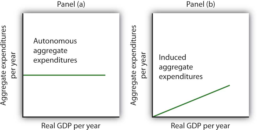
Autonomous aggregate expenditures do not vary with the level of real GDP; induced aggregate expenditures do. Autonomous aggregate expenditures are shown by the horizontal line in Panel (a). Induced aggregate expenditures vary with real GDP, as in Panel (b).
The concept of the marginal propensity to consume suggests that consumption contains induced aggregate expenditures; an increase in real GDP raises consumption. But consumption contains an autonomous component as well. The level of consumption at the intersection of the consumption function and the vertical axis is regarded as autonomous consumption; this level of spending would occur regardless of the level of real GDP.
Consider the consumption function we used in deriving the schedule and curve illustrated in Figure 13.2 "Plotting a Consumption Function":
We can omit the subscript on disposable personal income because of the simplifications we have made in this section, and the symbol Y can be thought of as representing both disposable personal income and GDP. Because we assume that the price level in the aggregate expenditures model is constant, GDP equals real GDP. At every level of real GDP, consumption includes $300 billion in autonomous aggregate expenditures. It will also contain expenditures “induced” by the level of real GDP. At a level of real GDP of $2,000 billion, for example, consumption equals $1,900 billion: $300 billion in autonomous aggregate expenditures and $1,600 billion in consumption induced by the $2,000 billion level of real GDP.
Figure 13.6 "Autonomous and Induced Consumption" illustrates these two components of consumption. Autonomous consumption, Ca, which is always $300 billion, is shown in Panel (a); its equation is
Equation 13.7
Induced consumption Ci is shown in Panel (b); its equation is
Equation 13.8
The consumption function is given by the sum of Equation 13.7 and Equation 13.8; it is shown in Panel (c) of Figure 13.6 "Autonomous and Induced Consumption". It is the same as the equation C = $300 billion + 0.8Yd, since in this simple example, Y and Yd are the same.
Figure 13.6 Autonomous and Induced Consumption
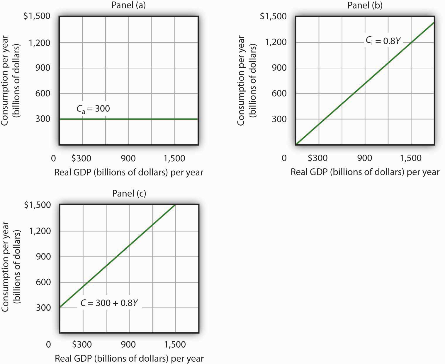
Consumption has an autonomous component and an induced component. In Panel (a), autonomous consumption Ca equals $300 billion at every level of real GDP. Panel (b) shows induced consumption Ci. Total consumption C is shown in Panel (c).
In this simplified economy, investment is the only other component of aggregate expenditures. We shall assume that investment is autonomous and that firms plan to invest $1,100 billion per year.
Equation 13.9
The level of planned investment is unaffected by the level of real GDP.
Aggregate expenditures equal the sum of consumption C and planned investment IP. The aggregate expenditures functionThe relationship of aggregate expenditures to the value of real GDP. is the relationship of aggregate expenditures to the value of real GDP. It can be represented with an equation, as a table, or as a curve.
We begin with the definition of aggregate expenditures AE when there is no government or foreign sector:
Equation 13.10
Substituting the information from above on consumption and planned investment yields (throughout this discussion all values are in billions of base-year dollars)
or
Equation 13.11
Equation 13.11 is the algebraic representation of the aggregate expenditures function. We shall use this equation to determine the equilibrium level of real GDP in the aggregate expenditures model. It is important to keep in mind that aggregate expenditures measure total planned spending at each level of real GDP (for any given price level). Real GDP is total production. Aggregate expenditures and real GDP need not be equal, and indeed will not be equal except when the economy is operating at its equilibrium level, as we will see in the next section.
In Equation 13.11, the autonomous component of aggregate expenditures is $1,400 billion, and the induced component is 0.8Y. We shall plot this aggregate expenditures function. To do so, we arbitrarily select various levels of real GDP and then use Equation 13.10 to compute aggregate expenditures at each level. At a level of real GDP of $6,000 billion, for example, aggregate expenditures equal $6,200 billion:
The table in Figure 13.7 "Plotting the Aggregate Expenditures Curve" shows the values of aggregate expenditures at various levels of real GDP. Based on these values, we plot the aggregate expenditures curve. To obtain each value for aggregate expenditures, we simply insert the corresponding value for real GDP into Equation 13.11. The value at which the aggregate expenditures curve intersects the vertical axis corresponds to the level of autonomous aggregate expenditures. In our example, autonomous aggregate expenditures equal $1,400 billion. That figure includes $1,100 billion in planned investment, which is assumed to be autonomous, and $300 billion in autonomous consumption expenditure.
Figure 13.7 Plotting the Aggregate Expenditures Curve
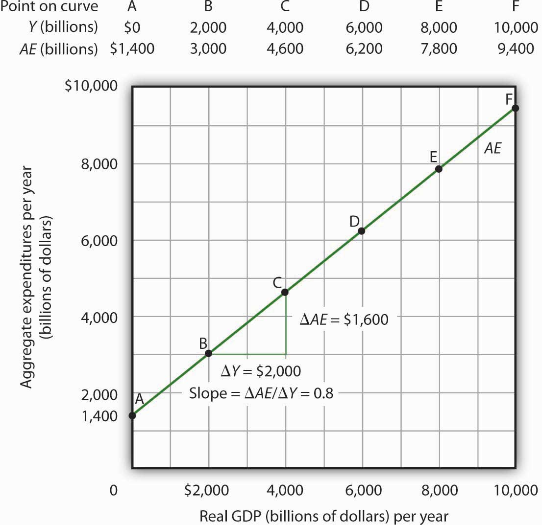
Values for aggregate expenditures AE are computed by inserting values for real GDP into Equation 13.10; these are given in the aggregate expenditures schedule. The point at which the aggregate expenditures curve intersects the vertical axis is the value of autonomous aggregate expenditures, here $1,400 billion. The slope of this aggregate expenditures curve is 0.8.
The slope of the aggregate expenditures curve, given by the change in aggregate expenditures divided by the change in real GDP between any two points, measures the additional expenditures induced by increases in real GDP. The slope for the aggregate expenditures curve in Figure 13.7 "Plotting the Aggregate Expenditures Curve" is shown for points B and C: it is 0.8.
In Figure 13.7 "Plotting the Aggregate Expenditures Curve", the slope of the aggregate expenditures curve equals the marginal propensity to consume. This is because we have assumed that the only other expenditure, planned investment, is autonomous and that real GDP and disposable personal income are identical. Changes in real GDP thus affect only consumption in this simplified economy.
Real GDP is a measure of the total output of firms. Aggregate expenditures equal total planned spending on that output. Equilibrium in the model occurs where aggregate expenditures in some period equal real GDP in that period. One way to think about equilibrium is to recognize that firms, except for some inventory that they plan to hold, produce goods and services with the intention of selling them. Aggregate expenditures consist of what people, firms, and government agencies plan to spend. If the economy is at its equilibrium real GDP, then firms are selling what they plan to sell (that is, there are no unplanned changes in inventories).
Figure 13.8 "Determining Equilibrium in the Aggregate Expenditures Model" illustrates the concept of equilibrium in the aggregate expenditures model. A 45-degree line connects all the points at which the values on the two axes, representing aggregate expenditures and real GDP, are equal. Equilibrium must occur at some point along this 45-degree line. The point at which the aggregate expenditures curve crosses the 45-degree line is the equilibrium real GDP, here achieved at a real GDP of $7,000 billion.
Figure 13.8 Determining Equilibrium in the Aggregate Expenditures Model
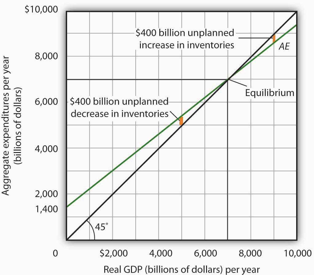
The 45-degree line shows all the points at which aggregate expenditures AE equal real GDP, as required for equilibrium. The equilibrium solution occurs where the AE curve crosses the 45-degree line, at a real GDP of $7,000 billion.
Equation 13.11 tells us that at a real GDP of $7,000 billion, the sum of consumption and planned investment is $7,000 billion—precisely the level of output firms produced. At that level of output, firms sell what they planned to sell and keep inventories that they planned to keep. A real GDP of $7,000 billion represents equilibrium in the sense that it generates an equal level of aggregate expenditures.
If firms were to produce a real GDP greater than $7,000 billion per year, aggregate expenditures would fall short of real GDP. At a level of real GDP of $9,000 billion per year, for example, aggregate expenditures equal $8,600 billion. Firms would be left with $400 billion worth of goods they intended to sell but did not. Their actual level of investment would be $400 billion greater than their planned level of investment. With those unsold goods on hand (that is, with an unplanned increase in inventories), firms would be likely to cut their output, moving the economy toward its equilibrium GDP of $7,000 billion. If firms were to produce $5,000 billion, aggregate expenditures would be $5,400 billion. Consumers and firms would demand more than was produced; firms would respond by reducing their inventories below the planned level (that is, there would be an unplanned decrease in inventories) and increasing their output in subsequent periods, again moving the economy toward its equilibrium real GDP of $7,000 billion. Figure 13.9 "Adjusting to Equilibrium Real GDP" shows possible levels of real GDP in the economy for the aggregate expenditures function illustrated in Figure 13.8 "Determining Equilibrium in the Aggregate Expenditures Model". It shows the level of aggregate expenditures at various levels of real GDP and the direction in which real GDP will change whenever AE does not equal real GDP. At any level of real GDP other than the equilibrium level, there is unplanned investment.
Figure 13.9 Adjusting to Equilibrium Real GDP
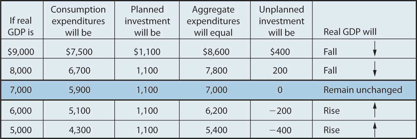
Each level of real GDP will result in a particular amount of aggregate expenditures. If aggregate expenditures are less than the level of real GDP, firms will reduce their output and real GDP will fall. If aggregate expenditures exceed real GDP, then firms will increase their output and real GDP will rise. If aggregate expenditures equal real GDP, then firms will leave their output unchanged; we have achieved equilibrium in the aggregate expenditures model. At equilibrium, there is no unplanned investment. Here, that occurs at a real GDP of $7,000 billion.
In the aggregate expenditures model, equilibrium is found at the level of real GDP at which the aggregate expenditures curve crosses the 45-degree line. It follows that a shift in the curve will change equilibrium real GDP. Here we will examine the magnitude of such changes.
Figure 13.10 "A Change in Autonomous Aggregate Expenditures Changes Equilibrium Real GDP" begins with the aggregate expenditures curve shown in Figure 13.8 "Determining Equilibrium in the Aggregate Expenditures Model". Now suppose that planned investment increases from the original value of $1,100 billion to a new value of $1,400 billion—an increase of $300 billion. This increase in planned investment shifts the aggregate expenditures curve upward by $300 billion, all other things unchanged. Notice, however, that the new aggregate expenditures curve intersects the 45-degree line at a real GDP of $8,500 billion. The $300 billion increase in planned investment has produced an increase in equilibrium real GDP of $1,500 billion.
Figure 13.10 A Change in Autonomous Aggregate Expenditures Changes Equilibrium Real GDP
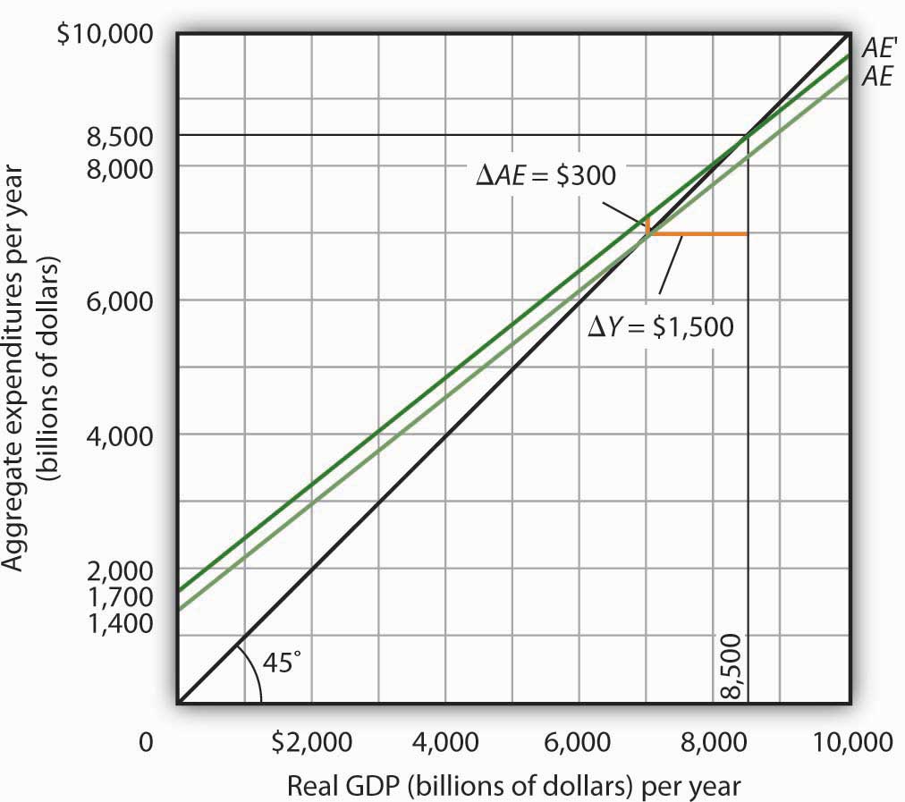
An increase of $300 billion in planned investment raises the aggregate expenditures curve by $300 billion. The $300 billion increase in planned investment results in an increase in equilibrium real GDP of $1,500 billion.
How could an increase in aggregate expenditures of $300 billion produce an increase in equilibrium real GDP of $1,500 billion? The answer lies in the operation of the multiplier. Because firms have increased their demand for investment goods (that is, for capital) by $300 billion, the firms that produce those goods will have $300 billion in additional orders. They will produce $300 billion in additional real GDP and, given our simplifying assumption, $300 billion in additional disposable personal income. But in this economy, each $1 of additional real GDP induces $0.80 in additional consumption. The $300 billion increase in autonomous aggregate expenditures initially induces $240 billion (= 0.8 × $300 billion) in additional consumption.
The $240 billion in additional consumption boosts production, creating another $240 billion in real GDP. But that second round of increase in real GDP induces $192 billion (= 0.8 × $240) in additional consumption, creating still more production, still more income, and still more consumption. Eventually (after many additional rounds of increases in induced consumption), the $300 billion increase in aggregate expenditures will result in a $1,500 billion increase in equilibrium real GDP. Table 13.1 "The Multiplied Effect of an Increase in Autonomous Aggregate Expenditures" shows the multiplied effect of a $300 billion increase in autonomous aggregate expenditures, assuming each $1 of additional real GDP induces $0.80 in additional consumption.
Table 13.1 The Multiplied Effect of an Increase in Autonomous Aggregate Expenditures
| Round of spending | Increase in real GDP (billions of dollars) |
|---|---|
| 1 | $300 |
| 2 | 240 |
| 3 | 192 |
| 4 | 154 |
| 5 | 123 |
| 6 | 98 |
| 7 | 79 |
| 8 | 63 |
| 9 | 50 |
| 10 | 40 |
| 11 | 32 |
| 12 | 26 |
| Subsequent rounds | +103 |
| Total increase in real GDP | $1,500 |
The size of the additional rounds of expenditure is based on the slope of the aggregate expenditures function, which in this example is simply the marginal propensity to consume. Had the slope been flatter (if the marginal propensity to consume were smaller), the additional rounds of spending would have been smaller. A steeper slope would mean that the additional rounds of spending would have been larger.
This process could also work in reverse. That is, a decrease in planned investment would lead to a multiplied decrease in real GDP. A reduction in planned investment would reduce the incomes of some households. They would reduce their consumption by the MPC times the reduction in their income. That, in turn, would reduce incomes for households that would have received the spending by the first group of households. The process continues, thus multiplying the impact of the reduction in aggregate expenditures resulting from the reduction in planned investment.
The multiplierThe number by which we multiply an initial change in aggregate demand to get the full amount of the shift in the aggregate demand curve. is the number by which we multiply an initial change in aggregate demand to get the full amount of the shift in the aggregate demand curve. Because the multiplier shows the amount by which the aggregate demand curve shifts at a given price level, and the aggregate expenditures model assumes a given price level, we can use the aggregate expenditures model to derive the multiplier explicitly.
Let Yeq be the equilibrium level of real GDP in the aggregate expenditures model, and let A be autonomous aggregate expenditures. Then the multiplier is
Equation 13.12
In the example we have just discussed, a change in autonomous aggregate expenditures of $300 billion produced a change in equilibrium real GDP of $1,500 billion. The value of the multiplier is therefore $1,500/$300 = 5.
The multiplier effect works because a change in autonomous aggregate expenditures causes a change in real GDP and disposable personal income, inducing a further change in the level of aggregate expenditures, which creates still more GDP and thus an even higher level of aggregate expenditures. The degree to which a given change in real GDP induces a change in aggregate expenditures is given in this simplified economy by the marginal propensity to consume, which, in this case, is the slope of the aggregate expenditures curve. The slope of the aggregate expenditures curve is thus linked to the size of the multiplier. We turn now to an investigation of the relationship between the marginal propensity to consume and the multiplier.
We can compute the multiplier for this simplified economy from the marginal propensity to consume. We know that the amount by which equilibrium real GDP will change as a result of a change in aggregate expenditures consists of two parts: the change in autonomous aggregate expenditures itself, , and the induced change in spending. This induced change equals the marginal propensity to consume times the change in equilibrium real GDP, ΔYeq. Thus
Equation 13.13
Subtract the MPCΔYeq term from both sides of the equation:
Factor out the ΔYeq term on the left:
Finally, solve for the multiplier by dividing both sides of the equation above by ΔA and by dividing both sides by (1 − MPC). We get the following:
Equation 13.14
We thus compute the multiplier by taking 1 minus the marginal propensity to consume, then dividing the result into 1. In our example, the marginal propensity to consume is 0.8; the multiplier is 5, as we have already seen [multiplier = 1/(1 − MPC) = 1/(1 − 0.8) = 1/0.2 = 5]. Since the sum of the marginal propensity to consume and the marginal propensity to save is 1, the denominator on the right-hand side of Equation 13.13 is equivalent to the MPS, and the multiplier could also be expressed as 1/MPS.
Equation 13.15
We can rearrange terms in Equation 13.14 to use the multiplier to compute the impact of a change in autonomous aggregate expenditures. We simply multiply both sides of the equation by to obtain the following:
Equation 13.16
The change in the equilibrium level of income in the aggregate expenditures model (remember that the model assumes a constant price level) equals the change in autonomous aggregate expenditures times the multiplier. Thus, the greater the multiplier, the greater will be the impact on income of a change in autonomous aggregate expenditures.
Four conclusions emerge from our application of the aggregate expenditures model to the simplified economy presented so far. These conclusions can be applied to a more realistic view of the economy.
These four points still hold as we add the two other components of aggregate expenditures—government purchases and net exports—and recognize that government not only spends but also collects taxes. We look first at the effect of adding taxes to the aggregate expenditures model and then at the effect of adding government purchases and net exports.
Suppose that the only difference between real GDP and disposable personal income is personal income taxes. Let us see what happens to the slope of the aggregate expenditures function.
As before, we assume that the marginal propensity to consume is 0.8, but we now add the assumption that income taxes take ¼ of real GDP. This means that for every additional $1 of real GDP, disposable personal income rises by $0.75 and, in turn, consumption rises by $0.60 (= 0.8 × $0.75). In the simplified model in which disposable personal income and real GDP were the same, an additional $1 of real GDP raised consumption by $0.80. The slope of the aggregate expenditures curve was 0.8, the marginal propensity to consume. Now, as a result of taxes, the aggregate expenditures curve will be flatter than the one shown in Figure 13.7 "Plotting the Aggregate Expenditures Curve" and Figure 13.9 "Adjusting to Equilibrium Real GDP". In this example, the slope will be 0.6; an additional $1 of real GDP will increase consumption by $0.60.
Other things the same, the multiplier will be smaller than it was in the simplified economy in which disposable personal income and real GDP were identical. The wedge between disposable personal income and real GDP created by taxes means that the additional rounds of spending induced by a change in autonomous aggregate expenditures will be smaller than if there were no taxes. Hence, the multiplied effect of any change in autonomous aggregate expenditures is smaller.
Suppose that government purchases and net exports are autonomous. If so, they enter the aggregate expenditures function in the same way that investment did. Compared to the simplified aggregate expenditures model, the aggregate expenditures curve shifts up by the amount of government purchases and net exports.An even more realistic view of the economy might assume that imports are induced, since as a country’s real GDP rises it will buy more goods and services, some of which will be imports. In that case, the slope of the aggregate expenditures curve would change.
Figure 13.11 "The Aggregate Expenditures Function: Comparison of a Simplified Economy and a More Realistic Economy" shows the difference between the aggregate expenditures model of the simplified economy in Figure 13.8 "Determining Equilibrium in the Aggregate Expenditures Model" and a more realistic view of the economy. Panel (a) shows an AE curve for an economy with only consumption and investment expenditures. In Panel (b), the AE curve includes all four components of aggregate expenditures.
Figure 13.11 The Aggregate Expenditures Function: Comparison of a Simplified Economy and a More Realistic Economy
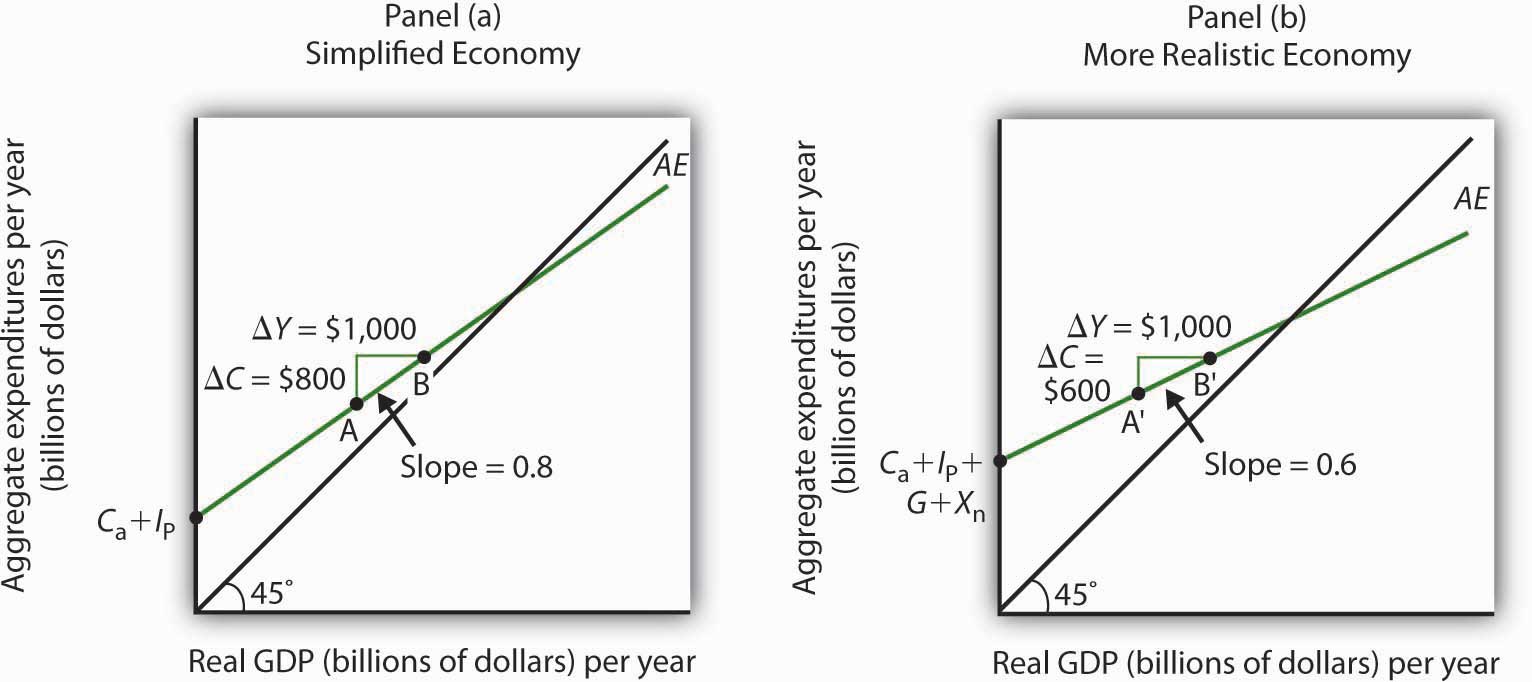
Panel (a) shows an aggregate expenditures curve for a simplified view of the economy; Panel (b) shows an aggregate expenditures curve for a more realistic model. The AE curve in Panel (b) has a higher intercept than the AE curve in Panel (a) because of the additional components of autonomous aggregate expenditures in a more realistic view of the economy. The slope of the AE curve in Panel (b) is flatter than the slope of the AE curve in Panel (a). In a simplified economy, the slope of the AE curve is the marginal propensity to consume (MPC). In a more realistic view of the economy, it is less than the MPC because of the difference between real GDP and disposable personal income.
There are two major differences between the aggregate expenditures curves shown in the two panels. Notice first that the intercept of the AE curve in Panel (b) is higher than that of the AE curve in Panel (a). The reason is that, in addition to the autonomous part of consumption and planned investment, there are two other components of aggregate expenditures—government purchases and net exports—that we have also assumed are autonomous. Thus, the intercept of the aggregate expenditures curve in Panel (b) is the sum of the four autonomous aggregate expenditures components: consumption (Ca), planned investment (IP), government purchases (G), and net exports (Xn). In Panel (a), the intercept includes only the first two components.
Second, notice that the slope of the aggregate expenditures curve is flatter for the more realistic economy in Panel (b) than it is for the simplified economy in Panel (a). This can be seen by comparing the slope of the aggregate expenditures curve between points A and B in Panel (a) to the slope of the aggregate expenditures curve between points A′ and B′ in Panel (b). Between both sets of points, real GDP changes by the same amount, $1,000 billion. In Panel (a), consumption rises by $800 billion, whereas in Panel (b) consumption rises by only $600 billion. This difference occurs because, in the more realistic view of the economy, households have only a fraction of real GDP available as disposable personal income. Thus, for a given change in real GDP, consumption rises by a smaller amount.
Let us examine what happens to equilibrium real GDP in each case if there is a shift in autonomous aggregate expenditures, such as an increase in planned investment, as shown in Figure 13.12 "A Change in Autonomous Aggregate Expenditures: Comparison of a Simplified Economy and a More Realistic Economy". In both panels, the initial level of equilibrium real GDP is the same, Y1. Equilibrium real GDP occurs where the given aggregate expenditures curve intersects the 45-degree line. The aggregate expenditures curve shifts up by the same amount—ΔA is the same in both panels. The new level of equilibrium real GDP occurs where the new AE curve intersects the 45-degree line. In Panel (a), we see that the new level of equilibrium real GDP rises to Y2, but in Panel (b) it rises only to Y3. Since the same change in autonomous aggregate expenditures led to a greater increase in equilibrium real GDP in Panel (a) than in Panel (b), the multiplier for the more realistic model of the economy must be smaller. The multiplier is smaller, of course, because the slope of the aggregate expenditures curve is flatter.
Figure 13.12 A Change in Autonomous Aggregate Expenditures: Comparison of a Simplified Economy and a More Realistic Economy
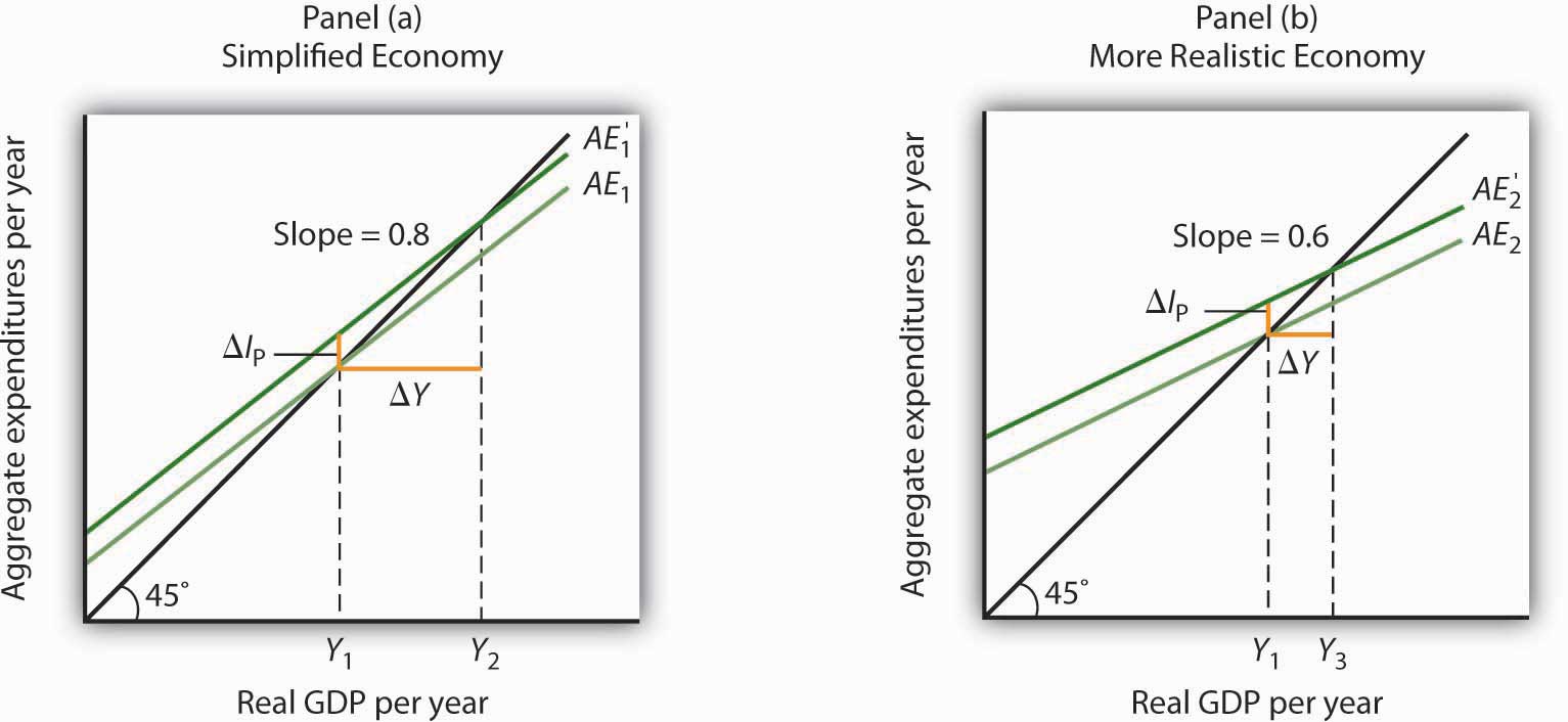
In Panels (a) and (b), equilibrium real GDP is initially Y1. Then autonomous aggregate expenditures rise by the same amount, ΔIP. In Panel (a), the upward shift in the AE curve leads to a new level of equilibrium real GDP of Y2; in Panel (b) equilibrium real GDP rises to Y3. Because equilibrium real GDP rises by more in Panel (a) than in Panel (b), the multiplier in the simplified economy is greater than in the more realistic one.
Suppose you are given the following data for an economy. All data are in billions of dollars. Y is actual real GDP, and C, IP, G, and Xn are the consumption, planned investment, government purchases, and net exports components of aggregate expenditures, respectively.
| Y | C | Ip | G | Xn |
|---|---|---|---|---|
| $0 | $800 | $1,000 | $1,400 | −$200 |
| 2,500 | 2,300 | 1,000 | 1,400 | −200 |
| 5,000 | 3,800 | 1,000 | 1,400 | −200 |
| 7,500 | 5,300 | 1,000 | 1,400 | −200 |
| 10,000 | 6,800 | 1,000 | 1,400 | −200 |

It was the first time expansionary fiscal policy had ever been proposed. The economy had slipped into a recession in 1960. Presidential candidate John Kennedy received proposals from several economists that year for a tax cut aimed at stimulating the economy. As a candidate, he was unconvinced. But, as president he proposed the tax cut in 1962. His chief economic adviser, Walter Heller, defended the tax cut idea before Congress and introduced what was politically a novel concept: the multiplier.
In testimony to the Senate Subcommittee on Employment and Manpower, Mr. Heller predicted that a $10 billion cut in personal income taxes would boost consumption “by over $9 billion.”
To assess the ultimate impact of the tax cut, Mr. Heller applied the aggregate expenditures model. He rounded the increased consumption off to $9 billion and explained,
“This is far from the end of the matter. The higher production of consumer goods to meet this extra spending would mean extra employment, higher payrolls, higher profits, and higher farm and professional and service incomes. This added purchasing power would generate still further increases in spending and incomes. … The initial rise of $9 billion, plus this extra consumption spending and extra output of consumer goods, would add over $18 billion to our annual GDP.”
We can summarize this continuing process by saying that a “multiplier” of approximately 2 has been applied to the direct increment of consumption spending.
Mr. Heller also predicted that proposed cuts in corporate income tax rates would increase investment by about $6 billion. The total change in autonomous aggregate expenditures would thus be $15 billion: $9 billion in consumption and $6 billion in investment. He predicted that the total increase in equilibrium GDP would be $30 billion, the amount the Council of Economic Advisers had estimated would be necessary to reach full employment.
In the end, the tax cut was not passed until 1964, after President Kennedy’s assassination in 1963. While the Council of Economic Advisers concluded that the tax cut had worked as advertised, it came long after the economy had recovered and tended to push the economy into an inflationary gap. As we will see in later chapters, the tax cut helped push the economy into a period of rising inflation.
Source: Economic Report of the President 1964 (Washington, DC: U.S. Government Printing Office, 1964), 172–73.
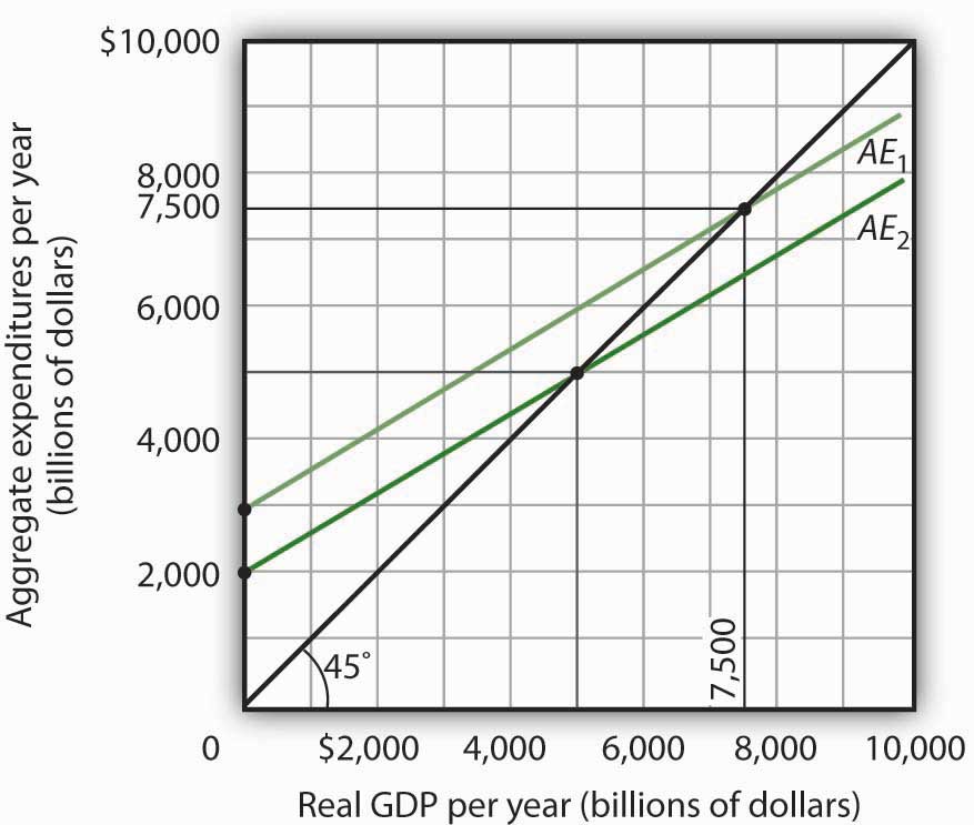
The intercept of the AE1 curve is $3,000. It is the amount of aggregate expenditures (C + IP + G + Xn) when real GDP is zero. The slope of the AE1 curve is 0.6. It can be found by determining the amount of aggregate expenditures for any two levels of real GDP and then by dividing the change in aggregate expenditures by the change in real GDP over the interval. For example, between real GDP of $2,500 and $5,000, aggregate expenditures go from $4,500 to $6,000. Thus,
We can use the aggregate expenditures model to gain greater insight into the aggregate demand curve. In this section we shall see how to derive the aggregate demand curve from the aggregate expenditures model. We shall also see how to apply the analysis of multiplier effects in the aggregate expenditures model to the aggregate demand–aggregate supply model.
An aggregate expenditures curve assumes a fixed price level. If the price level were to change, the levels of consumption, investment, and net exports would all change, producing a new aggregate expenditures curve and a new equilibrium solution in the aggregate expenditures model.
A change in the price level changes people’s real wealth. Suppose, for example, that your wealth includes $10,000 in a bond account. An increase in the price level would reduce the real value of this money, reduce your real wealth, and thus reduce your consumption. Similarly, a reduction in the price level would increase the real value of money holdings and thus increase real wealth and consumption. The tendency for price level changes to change real wealth and consumption is called the wealth effectThe tendency for price level changes to change real wealth and consumption..
Because changes in the price level also affect the real quantity of money, we can expect a change in the price level to change the interest rate. A reduction in the price level will increase the real quantity of money and thus lower the interest rate. A lower interest rate, all other things unchanged, will increase the level of investment. Similarly, a higher price level reduces the real quantity of money, raises interest rates, and reduces investment. This is called the interest rate effectThe tendency for a higher price level to reduce the real quantity of money, raise interest rates, and reduce investment..
Finally, a change in the domestic price level will affect exports and imports. A higher price level makes a country’s exports fall and imports rise, reducing net exports. A lower price level will increase exports and reduce imports, increasing net exports. This impact of different price levels on the level of net exports is called the international trade effectThe impact of different price levels on the level of net exports..
Panel (a) of Figure 13.13 "From Aggregate Expenditures to Aggregate Demand" shows three possible aggregate expenditures curves for three different price levels. For example, the aggregate expenditures curve labeled AEP=1.0 is the aggregate expenditures curve for an economy with a price level of 1.0. Since that aggregate expenditures curve crosses the 45-degree line at $6,000 billion, equilibrium real GDP is $6,000 billion at that price level. At a lower price level, aggregate expenditures would rise because of the wealth effect, the interest rate effect, and the international trade effect. Assume that at every level of real GDP, a reduction in the price level to 0.5 would boost aggregate expenditures by $2,000 billion to AEP = 0.5, and an increase in the price level from 1.0 to 1.5 would reduce aggregate expenditures by $2,000 billion. The aggregate expenditures curve for a price level of 1.5 is shown as AEP=1.5. There is a different aggregate expenditures curve, and a different level of equilibrium real GDP, for each of these three price levels. A price level of 1.5 produces equilibrium at point A, a price level of 1.0 does so at point B, and a price level of 0.5 does so at point C. More generally, there will be a different level of equilibrium real GDP for every price level; the higher the price level, the lower the equilibrium value of real GDP.
Figure 13.13 From Aggregate Expenditures to Aggregate Demand
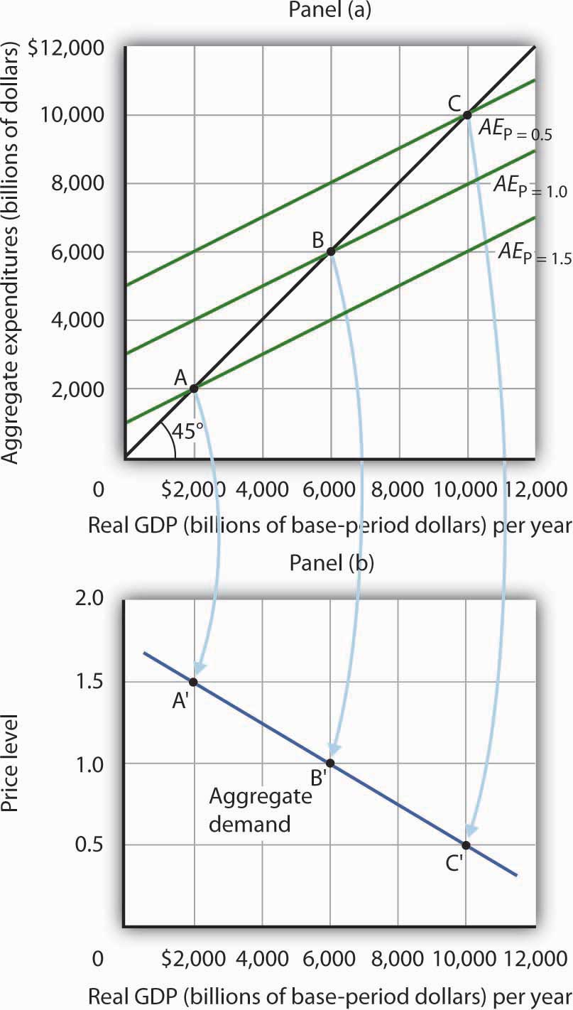
Because there is a different aggregate expenditures curve for each price level, there is a different equilibrium real GDP for each price level. Panel (a) shows aggregate expenditures curves for three different price levels. Panel (b) shows that the aggregate demand curve, which shows the quantity of goods and services demanded at each price level, can thus be derived from the aggregate expenditures model. The aggregate expenditures curve for a price level of 1.0, for example, intersects the 45-degree line in Panel (a) at point B, producing an equilibrium real GDP of $6,000 billion. We can thus plot point B′ on the aggregate demand curve in Panel (b), which shows that at a price level of 1.0, a real GDP of $6,000 billion is demanded.
Panel (b) of Figure 13.13 "From Aggregate Expenditures to Aggregate Demand" shows how an aggregate demand curve can be derived from the aggregate expenditures curves for different price levels. The equilibrium real GDP associated with each price level in the aggregate expenditures model is plotted as a point showing the price level and the quantity of goods and services demanded (measured as real GDP). At a price level of 1.0, for example, the equilibrium level of real GDP in the aggregate expenditures model in Panel (a) is $6,000 billion at point B. That means $6,000 billion worth of goods and services is demanded; point B' on the aggregate demand curve in Panel (b) corresponds to a real GDP demanded of $6,000 billion and a price level of 1.0. At a price level of 0.5 the equilibrium GDP demanded is $10,000 billion at point C', and at a price level of 1.5 the equilibrium real GDP demanded is $2,000 billion at point A'. The aggregate demand curve thus shows the equilibrium real GDP from the aggregate expenditures model at each price level.
In the aggregate expenditures model, a change in autonomous aggregate expenditures changes equilibrium real GDP by the multiplier times the change in autonomous aggregate expenditures. That model, however, assumes a constant price level. How can we incorporate the concept of the multiplier into the model of aggregate demand and aggregate supply?
Consider the aggregate expenditures curves given in Panel (a) of Figure 13.14 "Changes in Aggregate Demand", each of which corresponds to a particular price level. Suppose net exports rise by $1,000 billion. Such a change increases aggregate expenditures at each price level by $1,000 billion.
A $1,000-billion increase in net exports shifts each of the aggregate expenditures curves up by $1,000 billion, to AE′P=1.0 and AE′P=1.5. That changes the equilibrium real GDP associated with each price level; it thus shifts the aggregate demand curve to AD2 in Panel (b). In the aggregate expenditures model, equilibrium real GDP changes by an amount equal to the initial change in autonomous aggregate expenditures times the multiplier, so the aggregate demand curve shifts by the same amount. In this example, we assume the multiplier is 2. The aggregate demand curve thus shifts to the right by $2,000 billion, two times the $1,000-billion change in autonomous aggregate expenditures.
Figure 13.14 Changes in Aggregate Demand
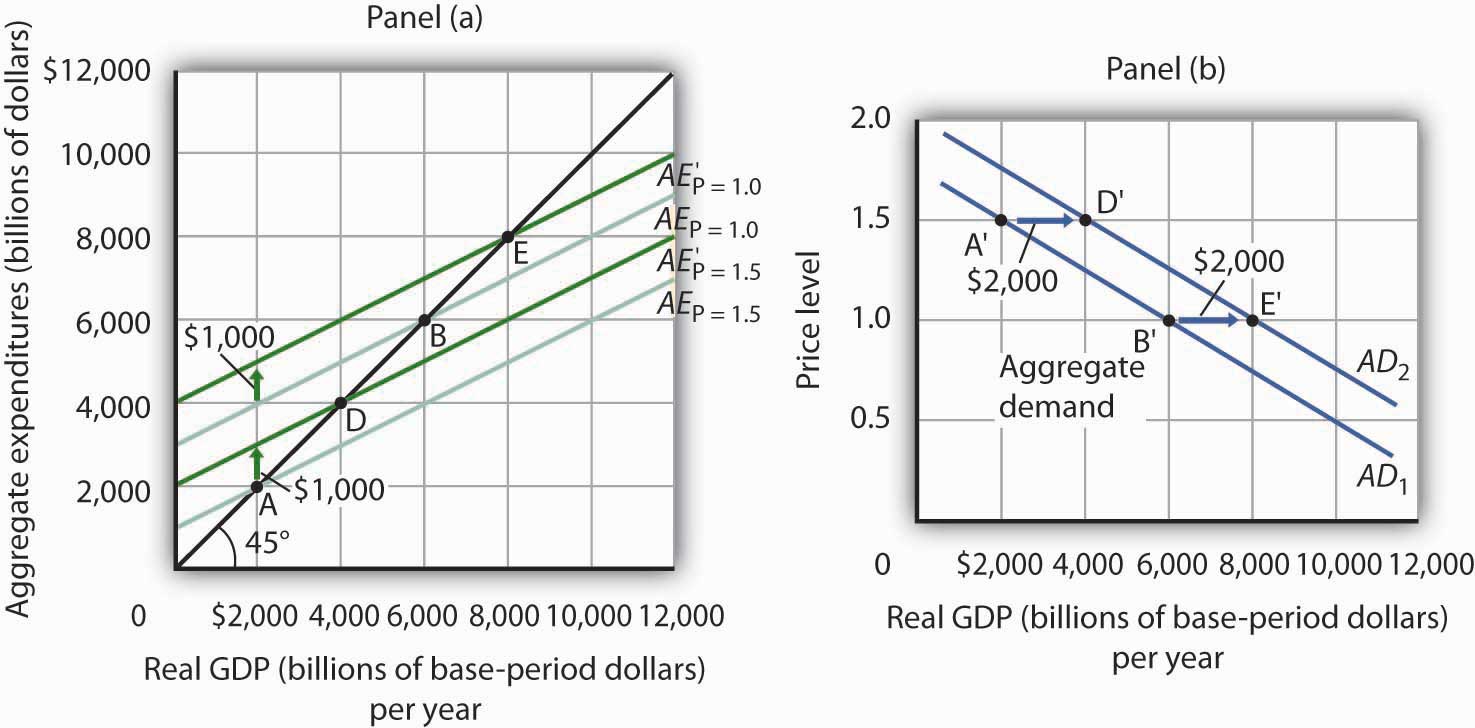
The aggregate expenditures curves for price levels of 1.0 and 1.5 are the same as in Figure 13.13 "From Aggregate Expenditures to Aggregate Demand", as is the aggregate demand curve. Now suppose a $1,000-billion increase in net exports shifts each of the aggregate expenditures curves up; AEP=1.0, for example, rises to AE′P=1.0. The aggregate demand curve thus shifts to the right by $2,000 billion, the change in aggregate expenditures times the multiplier, assumed to be 2 in this example.
In general, any change in autonomous aggregate expenditures shifts the aggregate demand curve. The amount of the shift is always equal to the change in autonomous aggregate expenditures times the multiplier. An increase in autonomous aggregate expenditures shifts the aggregate demand curve to the right; a reduction shifts it to the left.
Sketch three aggregate expenditures curves for price levels of P1, P2, and P3, where P1 is the lowest price level and P3 the highest (you do not have numbers for this exercise; simply sketch curves of the appropriate shape). Label the equilibrium levels of real GDP Y1, Y2, and Y3. Now draw the aggregate demand curve implied by your analysis, labeling points that correspond to P1, P2, and P3 and Y1, Y2, and Y3. You can use Figure 13.13 "From Aggregate Expenditures to Aggregate Demand" as a model for your work.

Using a large-scale model of the U.S. economy to simulate the effects of government policies, Princeton University professor Alan Blinder and Moody Analytics chief economist Mark Zandi concluded that the expansionary fiscal, monetary, and other policies aimed at relieving the financial crisis (such as the Troubled Asset Relief Program, or TARP) worked together from 2008 onward to effectively combat the Great Recession and probably kept it from turning into the Great Depression 2.0. Specifically, they estimated that U.S. GDP would have fallen about 12% peak-to-trough and that the unemployment rate would have hit 16.5% without these policies, instead of GDP declining about 4% and the unemployment rate reaching about 10%. While they attribute the bulk of the improvement to monetary and other financial policies, they found that fiscal policies also played a substantial role. For example, they concluded that fiscal stimulus added more than 3% to real GDP in 2010.
How much did the different components of the fiscal policies contribute? The following table provides estimates for the multiplied effects of various stimulus measures that were considered. In general, they estimate a stronger “bang for the buck,” or multiplier, from spending increases than from tax cuts.
| Tax cuts | Bang for the buck |
| Nonrefundable lump-sum tax rebate | 1.01 |
| Refundable lump-sum tax rebate | 1.22 |
| Temporary tax cuts | |
| Payroll tax holiday | 1.24 |
| Across-the-board tax cut | 1.02 |
| Accelerated depreciation | 0.25 |
| Permanent tax cuts | |
| Extend alternative minimum tax patch | 0.51 |
| Make Bush income tax cuts permanent | 0.32 |
| Make dividend and capital gains tax cuts permanent | 0.32 |
| Spending increases | |
| Extending UI benefits | 1.61 |
| Temporary increase in food stamps | 1.74 |
| General aid to state governments | 1.41 |
| Increased infrastructure spending | 1.57 |
While Blinder and Zandy acknowledge that no one can know for sure what would have happened without the policy responses and that not all aspects of the programs were perfectly designed or implemented, they feel strongly that the aggressive policies were, overall, appropriate and worth taking.
Source: Alan S. Blinder and Mark Zandi, “How the Great Recession Was Brought to an End,” Moody’s Economy.com, July 27, 2010.
The lowest price level, P1, corresponds to the highest AE curve, AEP = P1, as shown. This suggests a downward-sloping aggregate demand curve. Points A, B, and C on the AE curve correspond to points A′, B′, and C′ on the AD curve, respectively.

This chapter presented the aggregate expenditures model. Aggregate expenditures are the sum of planned levels of consumption, investment, government purchases, and net exports at a given price level. The aggregate expenditures model relates aggregate expenditures to the level of real GDP.
We began by observing the close relationship between consumption and disposable personal income. A consumption function shows this relationship. The saving function can be derived from the consumption function.
The time period over which income is considered to be a determinant of consumption is important. The current income hypothesis holds that consumption in one period is a function of income in that same period. The permanent income hypothesis holds that consumption in a period is a function of permanent income. An important implication of the permanent income hypothesis is that the marginal propensity to consume will be smaller for temporary than for permanent changes in disposable personal income.
Changes in real wealth and consumer expectations can affect the consumption function. Such changes shift the curve relating consumption to disposable personal income, the graphical representation of the consumption function; changes in disposable personal income do not shift the curve but cause movements along it.
An aggregate expenditures curve shows total planned expenditures at each level of real GDP. This curve is used in the aggregate expenditures model to determine the equilibrium real GDP (at a given price level). A change in autonomous aggregate expenditures produces a multiplier effect that leads to a larger change in equilibrium real GDP. In a simplified economy, with only consumption and investment expenditures, in which the slope of the aggregate expenditures curve is the marginal propensity to consume (MPC), the multiplier is equal to 1/(1 − MPC). Because the sum of the marginal propensity to consume and the marginal propensity to save (MPS) is 1, the multiplier in this simplified model is also equal to 1/MPS.
Finally, we derived the aggregate demand curve from the aggregate expenditures model. Each point on the aggregate demand curve corresponds to the equilibrium level of real GDP as derived in the aggregate expenditures model for each price level. The downward slope of the aggregate demand curve (and the shifting of the aggregate expenditures curve at each price level) reflects the wealth effect, the interest rate effect, and the international trade effect. A change in autonomous aggregate expenditures shifts the aggregate demand curve by an amount equal to the change in autonomous aggregate expenditures times the multiplier.
In a more realistic aggregate expenditures model that includes all four components of aggregate expenditures (consumption, investment, government purchases, and net exports), the slope of the aggregate expenditures curve shows the additional aggregate expenditures induced by increases in real GDP, and the size of the multiplier depends on the slope of the aggregate expenditures curve. The steeper the aggregate expenditures curve, the larger the multiplier; the flatter the aggregate expenditures curve, the smaller the multiplier.
Suppose the following information describes a simple economy. Figures are in billion of dollars.
| Disposable personal income | Consumption |
|---|---|
| 0 | 100 |
| 100 | 120 |
| 200 | 140 |
| 300 | 160 |
The graph below shows a consumption function.
For the purpose of this exercise, assume that the consumption function is given by C = $500 billion + 0.8Yd. Construct a consumption and saving table showing how income is divided between consumption and personal saving when disposable personal income (in billions) is $0, $500, $1,000, $1,500, $2,000, $2,500, $3,000, and $3,500.
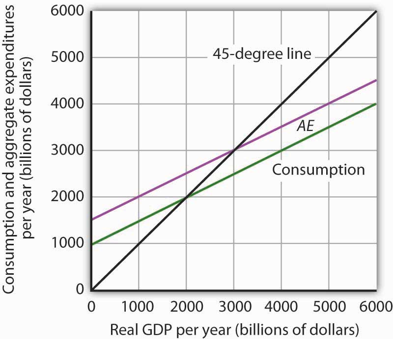
The graph below characterizes a simple economy with only two components of aggregate expenditures, consumption and investment.
Explain and illustrate graphically how each of the following events affects aggregate expenditures and equilibrium real GDP. In each case, state the nature of the change in aggregate expenditures, and state the relationship between the change in AE and the change in equilibrium real GDP.
The equations below give consumption functions for economies in which planned investment is autonomous and is the only other component of GDP. Compute the marginal propensity to consume and the multiplier for each economy.
Assume an economy in which people would spend $200 billion on consumption even if real GDP were zero and, in addition, increase their consumption by $0.50 for each additional $1 of real GDP. Assume further that the sum of planned investment plus government purchases plus net exports is $200 billion regardless of the level of real GDP.


