In this section we elaborate on the following:
Actuarial analysisA highly specialized mathematic analysis that deals with the financial and risk aspects of insurance. is a highly specialized mathematic analysis that deals with the financial and risk aspects of insurance. Actuarial analysis takes past losses and projects them into the future to determine the reserves an insurer needs to keep and the rates to charge. An actuaryIndividual who determines proper rates and reserves, certifies financial statements, participates in product development, and assists in overall management planning. determines proper rates and reserves, certifies financial statements, participates in product development, and assists in overall management planning.
Actuaries are expected to demonstrate technical expertise by passing the examinations required for admission into either the Society of Actuaries (for life/health actuaries) or the Casualty Actuarial Society (for property/casualty actuaries). Passing the examinations requires a high level of mathematical knowledge and skill.
The rates or premiums for insurance are based first and foremost on the past experience of losses. Actuaries calculate the rates using various procedures and techniques. The most modern techniques include sophisticated regression analysis and data mining tools. In essence, the actuary first has to estimate the expected claim payments (equaling the net premium) then “loads” the figure by factors meant to accommodate the underwriting, management, and claims handling expenses. In addition, other elements may be considered, such as a loading to cover the uncertainty element.
In some insurance lines (called long tail lines), claims are settled over a long period; therefore, the company must estimate its future payments before it can determine losses. The payments still pending and will be paid in the future are held as a liability for the insurance company and are called loss reserves or pending (or outstanding) losses. Typically, the claims department personnel give their estimates of the amounts that are expected to be paid for each open claim file, and the sum of these case by case estimates makes up the case estimates reserve. The actuaries offer their estimates based on sophisticated statistical analysis of aggregated data. Actuaries sometimes have to estimate, as a part of the loss reserves, the payments for claims that have not yet been reported as well. These incurred but not yet reported claims are referred to by the initials IBNR in industry parlance.
The loss reserves estimation is based on data of past claim payments. Such data is typically presented in the form of a triangle. Actuaries use many techniques to turn the triangle into a forecast. Some of the traditional, but still popular, methods are quite intuitive. For pedagogical reasons, we shall demonstrate one of those methods below. A more sophisticated and modern concept is presented in the appendix to this chapter (Section 7.4 "Appendix: Modern Loss Reserving Methods in Long Tail Lines") and reveals deficiencies of the traditional methods.
A hypothetical example of one loss-reserving technique is featured here in Table 7.1 "Incurred Losses for Accident Years by Development Periods (in Millions of Dollars)" through Table 7.5 "Development of the Triangle of Incurred Losses to Ultimate (in Millions of Dollars)". The technique used in these tables is known as a triangular method of loss development to the ultimate. The example is for illustration only. Loss developmentThe calculation of how amounts paid for losses increase (mature) over time for the purpose of future projection. is the calculation of how amounts paid for losses increase (or mature) over time for the purpose of future projection. Because the claims are paid progressively over time, like medical bills for an injury, the actuarial analysis has to project how losses will be developed into the future based on their past development.
With property/casualty lines such as product liability, the insurer’s losses can continue for many years after the initial occurrence of the accident. For example, someone who took certain weight-loss medications in 1994 (the “accident year”) might develop heart trouble six years later. Health problems from asbestos contact or tobacco use can occur decades after the accident actually occurred.
Table 7.1 "Incurred Losses for Accident Years by Development Periods (in Millions of Dollars)" describes an insurance company’s incurred losses for product liability from 1994 to 2000. Incurred lossesPaid losses plus known, but not yet paid losses. are both paid losses plus known but not yet paid losses. Look at accident year 1996: over the first twelve months after those accidents, the company posted losses of $38.901 million related to those accidents. Over the next twelve months—as more injuries came to light or belated claims were filed or lawsuits were settled—the insurer incurred almost $15 million, so that the cumulative losses after twenty-four developed months comes to $53.679 million. Each year brought more losses relating to accidents in 1996, so that by the end of the sixty-month development period, the company had accumulated $70.934 million in incurred losses for incidents from accident year 1996. The table ends there, but the incurred losses continue; the ultimate total is not yet known.
To calculate how much money must be kept in reserve for losses, actuaries must estimate the ultimate incurred loss for each accident year. They can do so by calculating the rate of growth of the losses for each year and then extending that rate to predict future losses. First, we calculate the rate for each development period. In accident year 1996, the $38.901 million loss in the first development period increased to $53.679 million in the second development period. The loss development factor for the twelve- to twenty-four-month period is therefore 1.380 million (53.679/38.901), meaning that the loss increased, or developed, by a factor of 1.380 (or 38 percent). The factor for twenty-four- to thirty-six months is 1.172 (62.904/53.679). The method to calculate all the factors follows the same pattern: the second period divided by first period. Table 7.2 "Loss Factors for Accident Years by Development Periods" shows the factors for each development period from Table 7.1 "Incurred Losses for Accident Years by Development Periods (in Millions of Dollars)".
Table 7.1 Incurred Losses for Accident Years by Development Periods (in Millions of Dollars)
| Developed Months | Accident Year | ||||||
|---|---|---|---|---|---|---|---|
| 1994 | 1995 | 1996 | 1997 | 1998 | 1999 | ||
| 12 | $37.654 | $38.781 | $38.901 | $36.980 | $37.684 | $39.087 | $37.680 |
| 24 | 53.901 | 53.789 | 53.679 | 47.854 | 47.091 | 47.890 | |
| 36 | 66.781 | 61.236 | 62.904 | 56.781 | 58.976 | ||
| 48 | 75.901 | 69.021 | 67.832 | 60.907 | |||
| 60 | 79.023 | 73.210 | 70.934 | ||||
| 72 | 81.905 | 79.087 | |||||
| 84 | 83.215 | ||||||
Table 7.2 Loss Factors for Accident Years by Development Periods
| Developed Months | Accident Year | |||||
|---|---|---|---|---|---|---|
| 1994 | 1995 | 1996 | 1997 | 1998 | ||
| 12–24 | 1.431 | 1.387 | 1.380 | 1.294 | 1.250 | 1.225 |
| 24–36 | 1.239 | 1.138 | 1.172 | 1.187 | 1.252 | |
| 36–48 | 1.137 | 1.127 | 1.078 | 1.073 | ||
| 48–60 | 1.041 | 1.061 | 1.046 | |||
| 60–72 | 1.036 | 1.080 | ||||
| 72–84 | 1.016 | |||||
| 84–ultimate | ||||||
After we complete the computation of all the factors in Table 7.2 "Loss Factors for Accident Years by Development Periods", we transpose the table in order to compute the averages for each development period. The transposed Table 7.2 "Loss Factors for Accident Years by Development Periods" is in Table 7.3 "Averages of the Incurred Loss Factors for Each Accident Year". The averages of the development factors are at the bottom of the table. You see, for example, that the average of factors for the thirty-six- to forty-eight-month development period of all accident years is 1.104. This means that, on average, losses increased by a factor of 1.104 (or 10.4 percent, if you prefer) in that period. That average is an ordinary mean. To exclude anomalies, however, actuaries often exclude the highest and lowest factors in each period, and average the remainders. The last line in Table 7.3 "Averages of the Incurred Loss Factors for Each Accident Year" is the average, excluding the high and low, and this average is used in Table 7.4 "Development of the Triangles of Incurred Loss Factors to Ultimate for Each Accident Year" to complete the triangle.
Table 7.3 Averages of the Incurred Loss Factors for Each Accident Year
| Accident Year | Developed Months | |||||
|---|---|---|---|---|---|---|
| 12–24 | 24–36 | 36–48 | 48–60 | 60–72 | ||
| 1994 | 1.431 | 1.239 | 1.137 | 1.041 | 1.036 | 1.016 |
| 1995 | 1.387 | 1.138 | 1.127 | 1.061 | 1.080 | |
| 1996 | 1.380 | 1.172 | 1.078 | 1.046 | ||
| 1997 | 1.294 | 1.187 | 1.073 | |||
| 1998 | 1.250 | 1.252 | ||||
| 1999 | 1.225 | |||||
| 12–24 | 24–36 | 36–48 | 48–60 | 60–72 | 72–84 | |
| Average | 1.328 | 1.198 | 1.104 | 1.049 | 1.058 | 1.016 |
| Average of last three years | 1.256 | 1.204 | 1.093 | 1.049 | 1.058 | 1.016 |
| Average of last four years | 1.287 | 1.187 | 1.104 | 1.049 | 1.058 | 1.016 |
| Average excluding high and low | 1.328 | 1.199 | 1.103 | 1.046 | 1.058 | 1.016 |
In Table 7.4 "Development of the Triangles of Incurred Loss Factors to Ultimate for Each Accident Year", we complete the incurred loss factors for the whole period of development. The information in bold is from Table 7.2 "Loss Factors for Accident Years by Development Periods". The information in italics is added for the later periods when incurred loss data are not yet available. These are the predictions of future losses. Thus, for accident year 1997, the bold part shows the factors from Table 7.2 "Loss Factors for Accident Years by Development Periods", which were derived from the actual incurred loss information in Table 7.1 "Incurred Losses for Accident Years by Development Periods (in Millions of Dollars)". We see from Table 7.4 "Development of the Triangles of Incurred Loss Factors to Ultimate for Each Accident Year" that we can expect losses to increase in any forty-eight- to sixty-month period by a factor of 1.046, in a sixty- to seventy-two-month period by 1.058, and in a seventy-two- to eighty-four-month period by 1.016. The development to ultimate factor is the product of all estimated factors: for 1997, it is 1.046 × 1.058 × 1.016 × 1.02 = 1.147. Actuaries adjust the development-to-ultimate factor based on their experience and other information.In this example, we do not introduce actuarial adjustments to the factors. Such adjustments are usually based on management, technology, marketing, and other known functional changes within the company. The book of business is assumed to be stable without any extreme changes that may require adjustments.
To determine ultimate losses, these factors can be applied to the dollar amounts in Table 7.1 "Incurred Losses for Accident Years by Development Periods (in Millions of Dollars)". Table 7.5 "Development of the Triangle of Incurred Losses to Ultimate (in Millions of Dollars)" provides the incurred loss estimates to ultimate payout for each accident year for this book of business. To illustrate how the computation is done, we estimate total incurred loss for accident year 1999. The most recent known incurred loss for accident year 1999 is as of 24 months: $47.890 million. To estimate the incurred losses at thirty-six months, we multiply by the development factor 1.199 and arrive at $57.426 million. That $57.426 million is multiplied by the applicable factors to produce a level of $63.326 million after forty-eight months, and $66.239 million after sixty months. Ultimately, the total payout for accident year 1999 is predicted to be $72.625 million. Because $47.890 million has already been paid out, the actuary will recommend keeping a reserve of $24.735 million to pay future claims. It is important to note that the ultimate level of incurred loss in this process includes incurred but not reported (IBNR) losses. Incurred but not reported (IBNR)Estimated losses that insureds did not claim yet but are expected to materialize in the future. losses are estimated losses that insureds did not claim yet, but they are expected to materialize in the future. This is usually an estimate that is hard to accurately project and is the reason the final projections of September 11, 2001, losses are still in question.
Table 7.4 Development of the Triangles of Incurred Loss Factors to Ultimate for Each Accident Year
| Developed Months | Accident Year | ||||||
|---|---|---|---|---|---|---|---|
| 1994 | 1995 | 1996 | 1997 | 1998 | 1999 | ||
| 12–24 | 1.431 | 1.387 | 1.380 | 1.294 | 1.250 | 1.225 | 1.328 |
| 24–36 | 1.239 | 1.138 | 1.172 | 1.187 | 1.252 | 1.199 | 1.199 |
| 36–48 | 1.137 | 1.127 | 1.078 | 1.073 | 1.103 | 1.103 | 1.103 |
| 48–60 | 1.041 | 1.061 | 1.046 | 1.046 | 1.046 | 1.046 | 1.046 |
| 60–72 | 1.036 | 1.080 | 1.058 | 1.058 | 1.058 | 1.058 | 1.058 |
| 72–84 | 1.016 | 1.016 | 1.016 | 1.016 | 1.016 | 1.016 | 1.016 |
| 84–ultimate* | 1.020 | 1.020 | 1.020 | 1.020 | 1.020 | 1.020 | 1.020 |
| Development to ultimate† | 1.020 | 1.036 | 1.096 | 1.147 | 1.265 | 1.517 | 2.014 |
| * Actuaries use their experience and other information to determine the factor that will be used from 84 months to ultimate. This factor is not available to them from the original triangle of losses. | |||||||
| † For example, the development to ultimate for 1997 is 1.046 × 1.058 × 1.016 × 1.02 = 1.147. | |||||||
Table 7.5 Development of the Triangle of Incurred Losses to Ultimate (in Millions of Dollars)
| Developed Months | Accident Year | |||||||
|---|---|---|---|---|---|---|---|---|
| 1994 | 1995 | 1996 | 1997 | 1998 | 1999 | 2000 | ||
| 12 | $37.654 | $38.781 | $38.901 | $36.980 | $37.684 | $39.087 | $37.680 | |
| 24 | 53.901 | 53.789 | 53.679 | 47.854 | 47.091 | 47.890 | 50.039 | |
| 36 | 66.781 | 61.236 | 62.904 | 56.781 | 58.976 | 57.426 | 60.003 | |
| 48 | 75.901 | 69.021 | 67.832 | 60.907 | 65.035 | 63.326 | 66.167 | |
| 60 | 79.023 | 73.210 | 70.934 | 63.709 | 68.027 | 66.239 | 69.211 | |
| 72 | 81.905 | 79.087 | 75.048 | 67.404 | 71.972 | 70.080 | 73.225 | |
| 84 | 83.215 | 80.352 | 76.249 | 68.482 | 73.123 | 71.201 | 74.396 | |
| Ultimate | 84.879 | 81.959 | 77.773 | 69.852 | 74.586 | 72.625 | 75.884 | 537.559 |
| Pd. to date | 83.215 | 79.087 | 70.934 | 60.907 | 58.976 | 47.890 | 37.680 | 438.689 |
| Reserve | 1.664 | 2.872 | 6.839 | 8.945 | 15.610 | 24.735 | 38.204 | 98.870 |
The process of loss development shown in the example of Table 7.1 "Incurred Losses for Accident Years by Development Periods (in Millions of Dollars)" through Table 7.5 "Development of the Triangle of Incurred Losses to Ultimate (in Millions of Dollars)" is used also for rate calculations because actuaries need to know the ultimate losses each book of business will incur. Rate calculationsThe computation of how much to charge for insurance coverage once the ultimate level of loss is estimated plus factors for taxes, expenses, and returns on investments. are the computations of how much to charge for insurance coverage once the ultimate level of loss is estimated, plus factors for taxes, expenses, and returns on investments.
Catastrophe (cat) modelingThe use of computer technology to synthesize loss data, assess historical disaster statistics, incorporate risk features, and run event simulations as an aid in predicting future losses. is composed of sophisticated statistical and technological mathematical equations and analysis that help predict future occurrences of natural and human-made disastrous events with large severity of losses. These models are relatively new and are made possible by the exponential improvements of information systems and statistical modeling over the years. Cat modeling relies on computer technology to synthesize loss data, assess historical disaster statistics, incorporate risk features, and run event simulations as an aid in predicting future losses. From this information, cat models project the impact of hypothetical catastrophes on residential and commercial properties.Claire Wilkinson, “Catastrophe Modeling: A Vital Tool in the Risk Management Box,” Insurance Information Institute, February 2008, Accessed March 6, 2009, http://www.iii.org/media/research/catmodeling/.
Cat modeling is concerned with predicting the future risk of catastrophes, primarily in the form of natural disasters. Cat modeling has its roots in the late 1980s and came to be utilized considerably following Hurricane Andrew in 1992 and the Northridge earthquake in 1994.Michael Lewis, “In Nature’s Casino,” New York Times Magazine, August 26, 2007, Accessed March 6, 2009; http://www.nytimes.com/2007/08/26/magazine/26neworleans-t.html. The parallel rapid sophistication of computer systems during this period was fortuitous and conducive to the growth of cat modeling. Today, every conceivable natural disaster is considered in cat models. Common hazard scenarios include hurricanes, earthquakes, tornados, and floods. One catastrophic event of increased concern in recent years is that of terrorism; some effort has been made to quantify the impact of this risk through cat models as well.AIR Worldwide, Accessed March 6, 2009, http://www.air-worldwide.com/ContentPage.aspx?id=16202.
Development of catastrophe models is complex, requiring the input of subject matter experts such as meteorologists, engineers, mathematicians, and actuaries. Due to the highly specialized nature and great demand for risk management tools, consulting firms have emerged to offer cat modeling solutions. The three biggest players in this arena are AIR Worldwide, Risk Management Solutions (RMS), and EQECAT.Claire Wilkinson, “Catastrophe Modeling: A Vital Tool in the Risk Management Box,” Insurance Information Institute, February 2008, Accessed March 6, 2009, http://www.iii.org/media/research/catmodeling/. The conclusions about exposures drawn from the models of different organizations are useful to insurers because they allow for better loss predictions of specific events.
Based on inputs regarding geographic locations, physical features of imperiled structures, and quantitative information about existing insurance coverage, catastrophe models render an output regarding the projected frequency, severity, and the overall dollar value of a catastrophic occurrence. From these results, it is possible to place property into appropriate risk categories. Thus, cat modeling can be extremely useful from an underwriting standpoint. Additionally, indications of high-dollar, high-severity risks in a particular region would certainly be influential to the development of premium rates and the insurer’s decision to explore reinsurance options (discussed in the next section of this chapter). Cat models are capable of estimating losses for a portfolio of insured properties.American Insurance Association, Testimony for the National Association of Insurance Commissioners (NAIC) 9/28/2007 Public Hearing on Catastrophe Modeling. Clearly, the interest that property/casualty insurers have in loss projections from hurricane catastrophes in southern Florida would benefit from this type of modeling.
Reliance on cat models came under fire following the devastating back-to-back hurricane seasons of 2004 and 2005. Critics argued that the models that were utilized underestimated the losses. It is important to note that the insurance industry is not the only market for cat models; consequently, different methodologies are employed depending on the needs of the end-user. These methodologies might incorporate different assumptions, inputs, and algorithms in calculation.Claire Wilkinson, “Catastrophe Modeling: A Vital Tool in the Risk Management Box,” Insurance Information Institute, February 2008, Accessed March 6, 2009, http://www.iii.org/media/research/catmodeling/. The unusually active 2004 and 2005 hurricane seasons could similarly be considered outside a normal standard deviation and thus unaccounted for by the models. In response to criticisms, refinements by developers following Hurricane Katrina included near-term projections providing probable maximum loss estimates using short-term expectations of hurricane activity.
For life insurance, actuaries use mortality tablesTables that indicate the percent of expected deaths for each age group., which predict the percentage of people in each age group who are expected to die each year. This percentage is used to estimate the required reserves and to compute life insurance rates. Life insurance, like other forms of insurance, is based on three concepts: pooling many exposures into a group, accumulating a fund paid for by contributions (premiums) from the members of the group, and paying from this fund for the losses of those who die each year. That is, life insurance involves the group sharing of individual losses. To set premium rates, the insurer must be able to calculate the probability of death at various ages among its insureds, based on pooling. Life insurers must collect enough premiums to cover mortality costs (the cost of claims). In addition to covering mortality costs, a life insurance premium, like a property/casualty premium, must reflect several adjustments, as noted in Table 7.6 "Term Premium Elements". The adjustments for various factors in life insurance premiums are known as premium elementsThe adjustments for various factors in life insurance premiums.. First, the premium is reduced because the insurer expects to earn investment incomeReturns from all the assets held by the insurers from both capital investment and from premiums., or returns from all the assets held by the insurers from both capital investment and from premiums. Investment is a very important aspect of the other side of the insurance business, as discussed below. Insurers invest the premiums they receive from insureds until losses need to be paid. Income from the investments is an offset in the premium calculations. By reducing the rates, most of an insurer’s investment income benefits consumers. Second, the premium is increased to cover the insurer’s marketing and administrative expenses, as described above. Taxes are the third component; those that are levied on the insurer also must be recovered. Fourth, in calculating premiums, an actuary usually increases the premium to cover the insurer’s risk of not predicting future losses accurately. The fifth element is the profits that the insurer should obtain because insurers are not “not for profit” organizations. All life insurance premium elements are depicted in Table 7.6 "Term Premium Elements" below. The actual prediction of deaths and the estimation of other premium elements are complicated actuarial processes.
Table 7.6 Term Premium Elements
| Mortality Cost |
|---|
| − Investment income |
| + Expense charge |
| + Taxes |
| + Risk change |
| + Profit |
| = Gross premium charge |
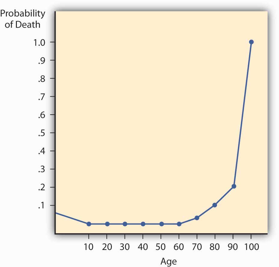
The mortality rate has two important characteristics that greatly influence insurer practices and the nature of life insurance contracts. First, yearly probabilities of death rise with age. Second, for practical reasons, actuaries set at 1.0 the probability of death at an advanced age, such as ninety-nine. That is, death during that year is considered a certainty, even though some people survive. The characteristics are illustrated with the mortality curve.
If we plot the probability of death for males by age, as in Figure 7.2 "Male Mortality Curve", we have a mortality curve. The mortality curveCurve that illustrates the relationship between age and the probability of death. illustrates the relationship between age and the probability of death. It shows that the mortality rate for males is relatively high at birth but declines until age ten. It then rises until age twenty-one and declines between ages twenty-two and twenty-nine. This decline apparently reflects many accidental deaths among males in their teens and early twenties, followed by a subsequent decrease. The rise is continuous for females older than age ten and for males after age twenty-nine. The rise is rather slow until middle age, at which point it begins to accelerate. At the more advanced ages, it rises very rapidly.
Figure 7.2 Male Mortality Curve
As noted above, insurance companies are in two businesses: the insurance business and the investment business. The insurance side is underwriting and reserving (liabilities), while the investment side is the area of securing the best rate of return on the assets entrusted to the insurer by the policyholders seeking the security. Investment income is a significant part of total income in most insurance companies. Liability accounts in the form of reserves are maintained on balance sheets to cover future claims and other obligations such as taxes and premium reserves. Assets must be maintained to cover the reserves and still leave the insurer with an adequate net worth in the form of capital and surplus. Capital and surplusThe equivalent of equity on the balance sheet of any firm—the net worth of the firm, or assets minus liabilities. are the equivalent of equity on the balance sheet of any firm—the net worth of the firm, or assets minus liabilities.
The investment mix of the life/health insurance industry is shown Table 7.7 "Life/Health Insurance Industry Asset Mix, 2003–2007 ($ Billions)" and that of the property/casualty industry is shown in Table 7.8 "Property/Casualty Insurance Industry Asset Mix, 2003–2007 ($ Billions)". As you can see, the assets of the life insurance industry in the United States were $4.95 trillion in 2007. This included majority investments in the credit markets, which includes bonds of all types and mortgage-backed securities of $387.5 billion. As discussed in Chapter 1 "The Nature of Risk: Losses and Opportunities" and the box below, “Problem Investments and the Credit Crisis,” many of these securities were no longer performing during the credit crisis of 2008–2009. In comparison, the U.S. property casualty industry’s asset holdings in 2007 were $1.37 trillion, with $125.8 billion in mortgage-backed securities. In Chapter 5 "The Evolution of Risk Management: Enterprise Risk Management", we included a discussion of risk management of the balance sheet to ensure that the net worth of the insurer is not lost when assets held are no longer performing. The capital and surplus of the U.S. property/casualty industry reached $531.3 billion at year-end 2007, up from $499.4 billion at year-end 2006. The capital and surplus of the U.S. life/health insurance industry was $252.8 billion in 2007, up from $244.4 billion in 2006.Insurance Information Institute. The Insurance Fact Book, 2009, p 31, 36.
Table 7.7 Life/Health Insurance Industry Asset Mix, 2003–2007 ($ Billions)
| Life/Health Insurer Financial Asset Distribution, 2003–2007 ($ Billions) | |||||
|---|---|---|---|---|---|
| 2003 | 2004 | 2005 | 2006 | 2007 | |
| Total financial assets | $3,772.8 | $4,130.3 | $4,350.7 | $4,685.3 | $4,950.3 |
| Checkable deposits and currency | 47.3 | 53.3 | 47.7 | 56.1 | 58.3 |
| Money market fund shares | 151.4 | 120.7 | 113.6 | 162.3 | 226.6 |
| Credit market instruments | 2,488.3 | 2,661.4 | 2,765.4 | 2,806.1 | 2,890.8 |
| Open market paper | 55.9 | 48.2 | 40.2 | 53.1 | 57.9 |
| U.S. government securities | 420.7 | 435.6 | 459.7 | 460.6 | 467.7 |
| Treasury | 71.8 | 78.5 | 91.2 | 83.2 | 80.2 |
| Agency and GSEGovernment-sponsored enterprise.-backed securities | 348.9 | 357.1 | 368.5 | 377.4 | 387.5 |
| Municipal securities | 26.1 | 30.1 | 32.5 | 36.6 | 35.3 |
| Corporate and foreign bonds | 1,620.2 | 1,768.0 | 1,840.7 | 1,841.9 | 1,889.7 |
| Policy loans | 104.5 | 106.1 | 106.9 | 110.2 | 113.9 |
| Mortgages | 260.9 | 273.3 | 285.5 | 303.8 | 326.2 |
| Corporate equities | 919.3 | 1,053.9 | 1,161.8 | 1,364.8 | 1,491.5 |
| Mutual fund shares | 91.7 | 114.4 | 109.0 | 148.8 | 161.4 |
| Miscellaneous assets | 74.7 | 126.6 | 153.1 | 147.1 | 121.6 |
| Source: Board of Governors of the Federal Reserve System, June 5, 2008. | |||||
Source: Insurance Information Institute, Accessed March 6, 2009, http://www.iii.org/media/facts/statsbyissue/life/.
Table 7.8 Property/Casualty Insurance Industry Asset Mix, 2003–2007 ($ Billions)
| Property/Casualty Insurer Financial Asset Distribution, 2003–2007 ($ Billions) | |||||
|---|---|---|---|---|---|
| 2003 | 2004 | 2005 | 2006 | 2007 | |
| Total financial assets | $1,059.7 | $1,162.2 | $1,243.8 | $1,329.3 | $1,373.6 |
| Checkable deposits and currency | 34.6 | 25.9 | 21.0 | 29.9 | 42.7 |
| Security repurchase agreementsShort-term agreements to sell and repurchase government securities by a specified date at a set price. | 52.8 | 63.1 | 68.9 | 66.0 | 53.8 |
| Credit market instruments | 625.2 | 698.8 | 765.8 | 813.5 | 840.0 |
| U.S. government securities | 180.1 | 183.4 | 187.1 | 197.8 | 180.9 |
| Treasury | 64.7 | 71.3 | 69.2 | 75.8 | 55.1 |
| Agency and GSEGovernment-sponsored enterprise.-backed securities | 115.4 | 112.1 | 117.9 | 122.0 | 125.8 |
| Municipal securities | 224.2 | 267.8 | 313.2 | 335.2 | 368.7 |
| Corporate and foreign bonds | 218.9 | 245.3 | 262.8 | 277.0 | 285.6 |
| Commercial mortgages | 2.1 | 2.4 | 2.7 | 3.5 | 4.8 |
| Corporate equities | 178.4 | 196.6 | 199.5 | 227.0 | 235.3 |
| Trade receivables | 79.3 | 79.6 | 82.1 | 87.0 | 85.4 |
| Miscellaneous assets | 85.0 | 93.0 | 100.7 | 99.0 | 108.7 |
| Source: Board of Governors of the Federal Reserve System, June 5, 2008. | |||||
Source: Insurance Information Institute, Accessed March 6, 2009, http://www.iii.org/media/facts/statsbyissue/life/.
The liabilities are composed mostly of reserves for loss payments. For the life insurance industry, the largest component of liabilities is reserves for pensions. Life reserves are the second-largest component. For property/casualty insurers, the reserves are for all lines of insurance, depending on the mix of products sold by each company.
Many conglomerate insurance corporations own their own investment firms and provide mutual funds. In this area, insurers, like other financial institutions, are subject to regulation by the states and by the Securities and Exchange Commission.
The greater risk faced by insurance companies is not the threat of going out of business due to insufficient sales volume, but the possibility that losses will be greater than anticipated and that they won’t be covered through reserves and investment income. This further reinforces the importance of comprehending the nature of insureds’ business and properly categorizing their risks on the underwriting side, while accurately capturing loss expectations on the actuarial side. Insuring common risks in high volume leads to more accuracy in predicting losses, but these risks do not vanish simply because they have been aggregated by the insurer. Unfortunately, this concept was not taken into consideration by several large investment banks and some insurance companies during the credit crisis beginning in 2007.
The credit crisis began when the U.S, housing bubble burst, setting off a protracted period characterized by increased valuation in real property, low interest rates, speculative investing, and massive demand for homes. During the housing bubble, low interest rates coupled with high liquidity were viewed as sufficiently favorable conditions to permit the extension of credit to high-risk (or subprime) borrowers. Many people who would otherwise not qualify for loans found themselves with mortgages and the homes of their dreams. Lenders protected themselves through the issuance of variable interest rate mortgages, whereby increased risk could be transferred to borrowers in the form of interest rate hikes. While this had the potential to put already high-risk (subprime) borrowers in an even worse position to meet their monthly obligations, borrowers counted on the very liquid nature of real estate during this period as a crutch to salvage their investments. Because home valuations and turnover were rising at such rapid rates, it was reasoned that financially strapped borrowers could simply sell and pay off their mortgages rather than face foreclosure.
The cycle of high turnover feeding into the housing bubble was halted when excess inventory of new homes and interest rate increases led to a downward correction of housing prices in 2005.“Getting worried downtown.” The Economist November 15, 2007. When lenders tried to pass these rate increases on to their buyers—many of whom had put little money down and had lived in their homes for less than a year—mortgage payments skyrocketed, even to the point of leaving buyers owing more than their homes were worth (negative equity). Home buying activity thus halted, leaving real estate a highly illiquid investment. The worst-case scenario was materializing, with foreclosures leaping to a staggering 79 percent in 2007, comprised of about 1.3 million homes.“U.S Foreclosure Activity Increases 75 Percent in 2007,” RealtyTrac, January 29, 2008, Accessed March 6, 2009, http://www.realtytrac.com/ContentManagement/pressrelease.aspx?ChannelID=9&ItemID=3988&accnt=64847.
During the housing bubble, the concept of risk transfer was carried out to an egregious extent. Lenders recognized the inherent riskiness of their activities, but they compounded the problem by attempting to transfer this risk to the very source of it. In other cases, subprime loans were sold to investment banks, who bundled them into exotic investment vehicles known as mortgage-backed securities (MBSs). These securities, derived mainly from subprime mortgages, ordinarily would be comparable to junk bonds in their risk assessment. Nevertheless, by dividing them into different investment classifications and purchasing credit-default swap (CDS) insurance (discussed below), investment banks were able to acquire acceptable grades on MBSs from the major rating agencies.“Let the Blame Begin; Everyone Played Some Role—The Street, Lenders, Ratings Agencies, Hedge Funds, Even Homeowners. Where Does Responsibility Lie? (The Subprime Mess),” Business Week Online, July 30, 2007. Investment-grade MBSs were in turn marketed as collateralized debt obligations (CDOs) and other options and sold to institutional investors. Ultimately, this group was left holding the bag when foreclosures rippled through the system, rendering the derivative investments worthless. Thus, the lending pendulum swung in the opposite direction, making it difficult for normally creditworthy borrowers to secure even rudimentary business loans. The pass-the-buck mentality with respect to risk transfer precipitated this credit crunch, which came to be known as the credit crisis. Everyone wanted the risky mortgage-backed securities off their balance sheets without acknowledging the potential folly of investing in them in the first place.
As it relates to the insurance industry, recall that insurers must hold assets that are sufficient to cover their liabilities (as discussed in the previous section) at any given time. In much the same way that a mortgage holder is required to purchase mortgage insurance to protect the lender when equity accounts for less than 25 percent of the total value of his or her home, issuers of MBSs engage in what are called credit default swaps (CDSs) to reassure investors.“The Financial Meltdown of AIG and Insurers Explained.” Smallcap Network, October 27, 2008, http://www.smallcapnetwork.com/scb/the-financial-meltdown-of-aig-and-other-insurers-explained/2315/. Insuring CDSs means that an insurer, rather than the MBS issuer, will deliver the promised payment to MBS investors in the event of default (in this case, foreclosure of the underlying mortgages).
AIG was one of the largest issuers of CDS insurance at the time of the credit crisis. The tightening of standards with respect to risk forced CDS insurers like AIG to hold liquid assets such that payouts could be made in the event that all of their CDS writings made claims. To illustrate, this burden would be the equivalent of all of a company’s insured homeowners suffering total losses simultaneously. While this scenario was improbable, the capital had to be set aside as if it would occur. AIG found it impossible to shore up enough assets to match against its now enormous liabilities, plunging the company into dire financial straits. In September 2008, AIG was extended an $85 billion line of credit from the Federal Reserve,Edmund L. Andrews, Michael J. de la Merced, and Mary Williams Walsh, “Fed’s $85 Billion Loan Rescues Insurer,” The New York Times, September 17, 2008, Accessed March 6, 2009, http://www.nytimes.com/2008/09/17/business/17insure.html. adding to the list of companies bailed out by the U.S. government in the wake of the economic recession brought about by the credit crisis.
At the Senate Budget Committee hearing on March 2, 2009, Federal Reserve Board Chairman Ben Bernanke testified as to the role of failures in the regulatory environment that allowed AIG to accumulate so much bad debt on its books. Bernanke accused the company of exploiting the fact that there was no oversight of the financial products division and went on to say, “If there’s a single episode in this entire 18 months that has made me more angry [than AIG], I can’t think of one.” He likened AIG to a “hedge fund … attached to a large and stable insurance company” that made “irresponsible bets” in explaining the firm’s actions leading up to its financial meltdown. Bernanke called for the Obama administration to expand the powers of the Federal Deposit Insurance Corporation (FDIC) to address the problems of large financial institutions rather than focusing on banks alone.Arthur D. Postal, “Fed Chief Blasts AIG for Exploiting Reg System,” National Underwriter Online, Property/Casualty Edition, March 3, 2009, Accessed March 6, 2009. http://www.propertyandcasualtyinsurancenews.com/cms/nupc/Breaking+News/2009/03/03-AIG-HEARING-dp.
In this section you studied the following:
The following table shows the incurred losses of the Maruri Insurance Company for its liability line.
| Development Months | Accident Year | ||||||
|---|---|---|---|---|---|---|---|
| 1994 | 1995 | 1996 | 1997 | 1998 | 1999 | ||
| 12 | $27,634 | $28,781 | $28,901 | $26,980 | $27,684 | $29,087 | $27,680 |
| 24 | $43,901 | $43,777 | $43,653 | $37,854 | $37,091 | $37,890 | |
| 36 | $56,799 | $51,236 | $52,904 | $46,777 | $48,923 | ||
| 48 | $65,901 | $59,021 | $57,832 | $50,907 | |||
| 60 | $69,023 | $63,210 | $60,934 | ||||
| 72 | $71,905 | $69,087 | |||||
| 84 | $73,215 | ||||||
Using the example in this chapter as a guide, do the following:
Read Section 7.4 "Appendix: Modern Loss Reserving Methods in Long Tail Lines" and respond to the following:
The table below shows the cumulative claim payments of the Enlightened Insurance Company for its liability line.
| Development Year | |||||||
|---|---|---|---|---|---|---|---|
| Accident Year | 0 | 1 | 2 | 3 | 4 | 5 | 6 |
| 2002 | $27,634 | $28,781 | $28,901 | $26,980 | $27,684 | $29,087 | $27,680 |
| 2003 | $43,901 | $43,777 | $43,653 | $37,854 | $37,091 | $37,890 | |
| 2004 | $56,799 | $51,236 | $52,904 | $46,777 | $48,923 | ||
| 2005 | $65,901 | $59,021 | $57,832 | $50,907 | |||
| 2006 | $69,023 | $63,210 | $60,934 | ||||
| 2007 | $71,905 | $69,087 | |||||
| 2008 | $73,215 | ||||||


