Many businesses need a loan in order to cover startup costsThese are fixed costs associated with starting a business. Often refers to one time costs.. Many entrepreneurs will turn to family for a loan. However, the danger here is that you are risking not only your family’s money, but also the relationships if the business should go under.
On the other hand, small businesses without a prior track record sometimes have trouble securing a bank loan. Fortunately, there are government agencies at both the federal and state levels that help businesses secure grants and loans.
Loan payments form part of the fixed costs of a business. Determining the payments on a loan is an important part of forecasting costs. The financial formula that calculates loan payments is fairly complex. However, Excel provides an easier way to calculate loan payments using the payment (PMT) functionA built in Excel function that calculates loan payments. Inputs to the function include the loan amount (pv), the interest rate (rate), and the number of loan payments (nper).. The PMT function is one of many built in Excel functions. In this chapter we will examine functions, how they differ from formulas, and how to use them in a spreadsheet.
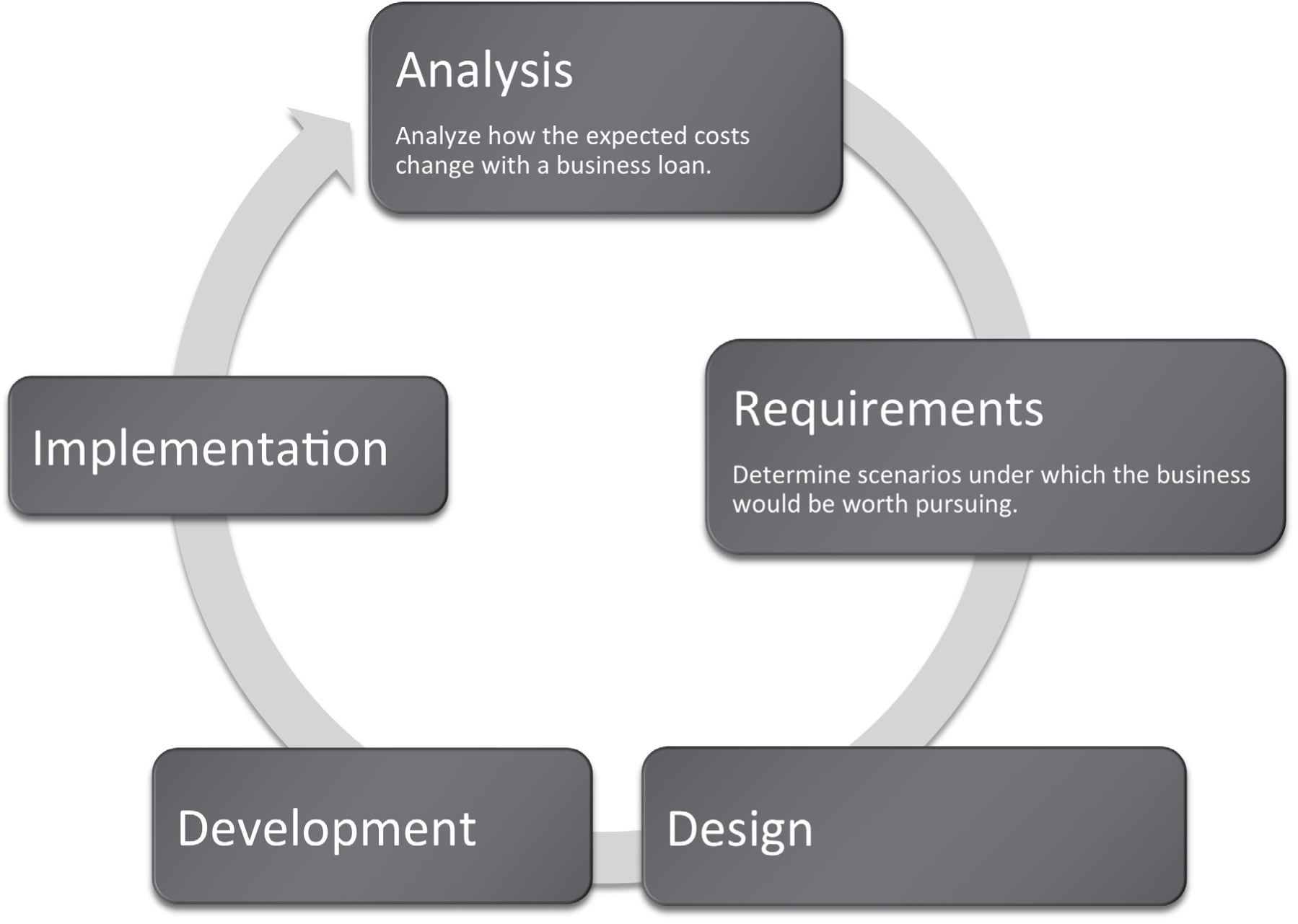
Many information systems projects are conceived of in a life cycle that progresses in stages from analysis to implementation. The diagram below shows the stages that we touch in the current chapter:
In the prior chapter we looked at Excel formulas and how to construct them. In many cases, we want to create our own formulas so we have a clear idea of how the information is constructed.
However, in some cases the formula might involve more complex math where the possibility for error is greater. In these cases it is better to use a built in functionA function is similar to a stored formula. However, functions usually hide details of the formula from the user. For example, we can use the PMT function to calculate loan payments without ever knowing the mathematical formula behind the function. that has already been tested and debugged. There are also functions that avoid busywork that you could do yourself but would probably prefer not to do.
On a small scale this is analogous to the build vs. buy issue. Think of formulas as things that you build whereas functions are things that you “buy.” We put buy in quotes because many functions, including the payment function, are bundled with Excel. That is part of the way that Excel maintains its leadership in the spreadsheet marketplace.
Most functions process input to produce a result. Perhaps the most popular function in Excel is the sum (SUM) functionAlso represented by Σ, the sum function adds up a column or row of numbers., which adds up a long list of numbers. The input for the Sum function are the cells to be added together.
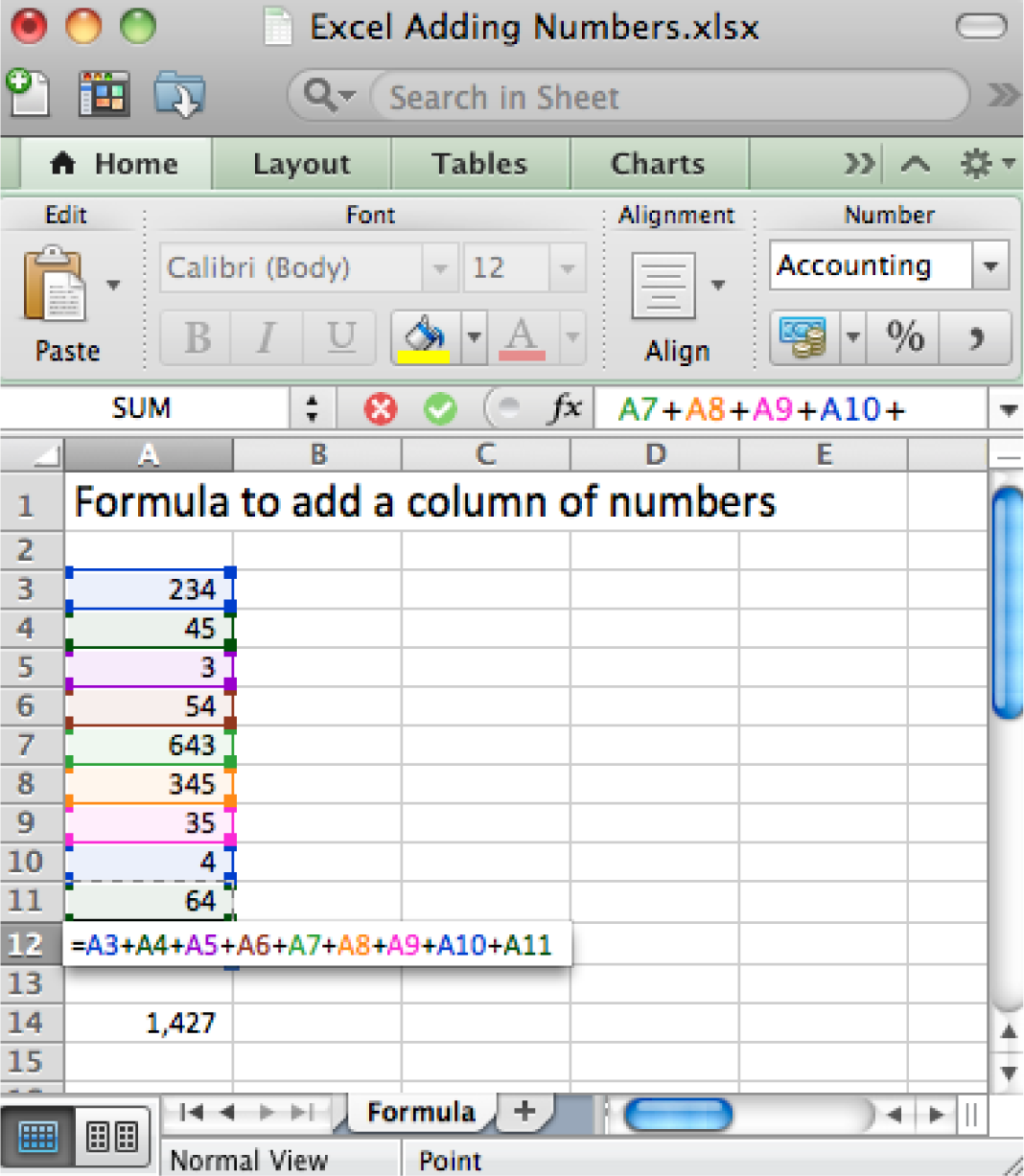
The example below shows the sum function compared with the equivalent formula. The formula is obviously very tedious as it involves adding all the numbers. This is expressed as
=A4+A5+A6+A7+A8+A9+A10+A11+A12The sum function accomplishes the same task more simplistically. This is expressed as
=SUM(A4:A12)Note that in both cases the result is the same: 1,427.
One nice advantage of the sum function is that if we were to add a row in the middle of the list, say between row 7 and row 8, the sum function would automatically expand to accommodate the new row, but the formula would not.
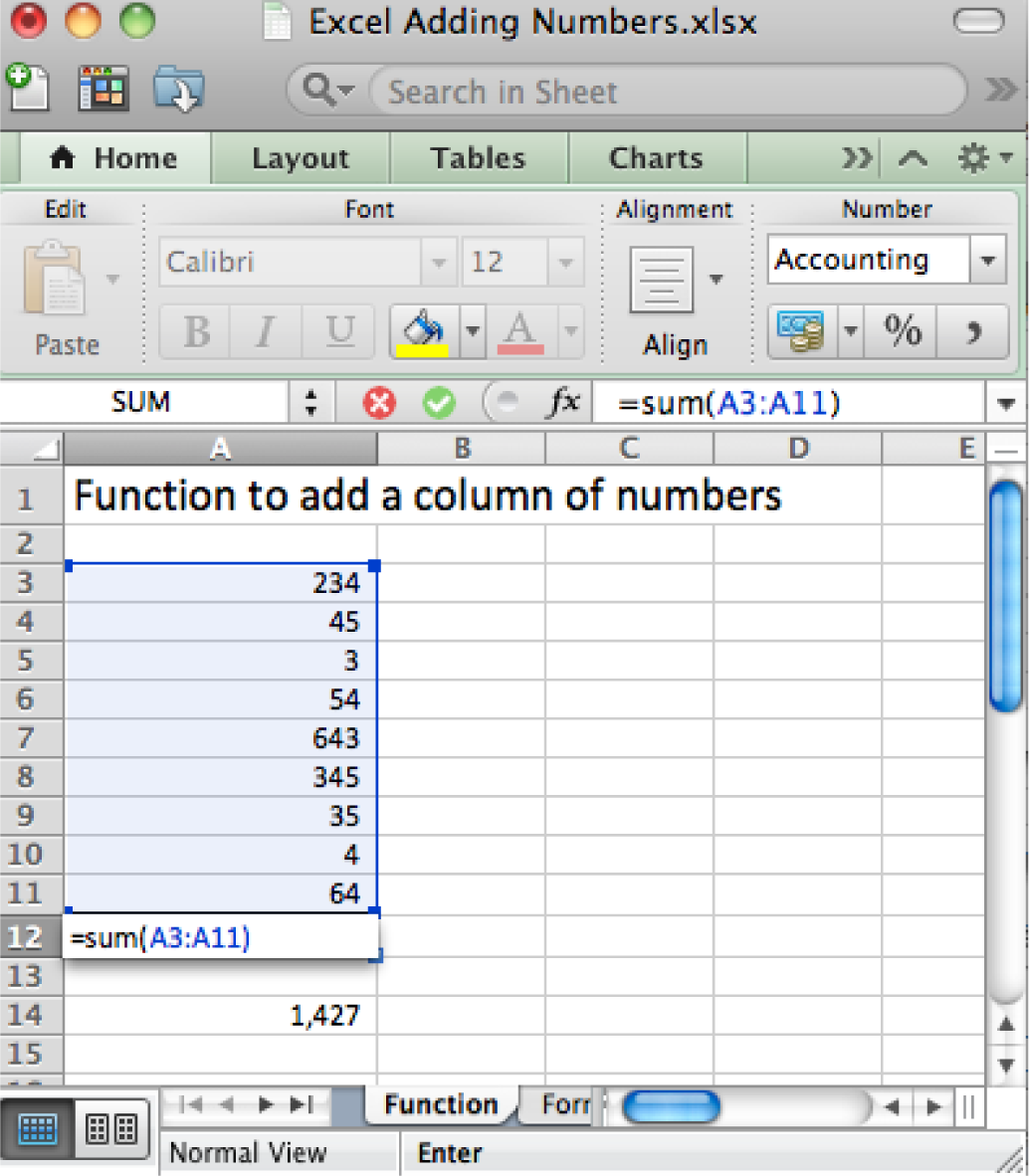
The right way (above) and wrong way (below) to add up a column of numbers. Always try to use the sum function when adding numbers from more than two cells.
The payment (PMT) function calculates loan payments automatically. The format of the PMT function is:
=PMT(rate,nper,pv) correct for YEARLY paymentsAdjusting for monthly payments produces this modification of the function:
=PMT(rate/12,nper*12,pv) correct for MONTHLY paymentsBy the way, you can use the PMT function to calculate payments on car loans and home mortgages. In case you are curious, the actual mathematical formula that the PMT function translates to looks like this:
Payment = pv* apr/12*(1+apr/12)^(nper*12)/((1+apr/12)^(nper*12)-1)Note that it is hard to even follow a complex mathematical formula when it is written in Excel.
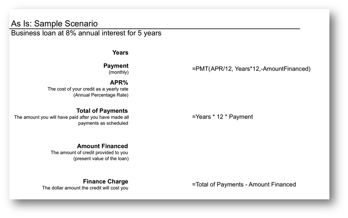
The payment (PMT) function in action. The wording in this illustration is taken directly from U.S. federal guidelines for loan disclosure. The PMT function is used to calculate the monthly payment—in this case $101. The function references three other numbers in the same illustration. Years is multiplied by 12 to get the number of payments (nper), APR% is divided by 12 to get the monthly interest rate, Amount Financed is the present value (pv) of the loan—the amount you are borrowing.
In the United States, the federal government places requirements on the actual wording of a loan. This wording is reflected in the illustration below. The intention is to force lenders to be honest about the terms of the loan and to allow buyers to comparison shop loans.
Note especially the finance chargeThe total interest paid over the life of the loan. The finance charge is calculated by adding up all of the loan payments and then subtracting from this total the amount originally borrowed. . This number is what people normally understand to be interest on the loan. It is the cost you pay for the privilege of borrowing the money. Now you might be wondering why this number is so high. After all 8% of $5,000 is only $400 not $1,083. The interest compounds or grows because the loan has been stretched out over five years.
First time home buyers are often shocked to find that their finance charge actually exceeds the amount of the loan. In other words, over the life of the loan they end up paying around twice the closing price of the home. Home loans have higher finance charges because they are often stretched out over thirty years—which is a lot of time to compound interest. Similarly, if we were to stretch our $5,000 business loan out over thirty years, the finance charge climbs to $8,208, which exceeds the amount of the loan.
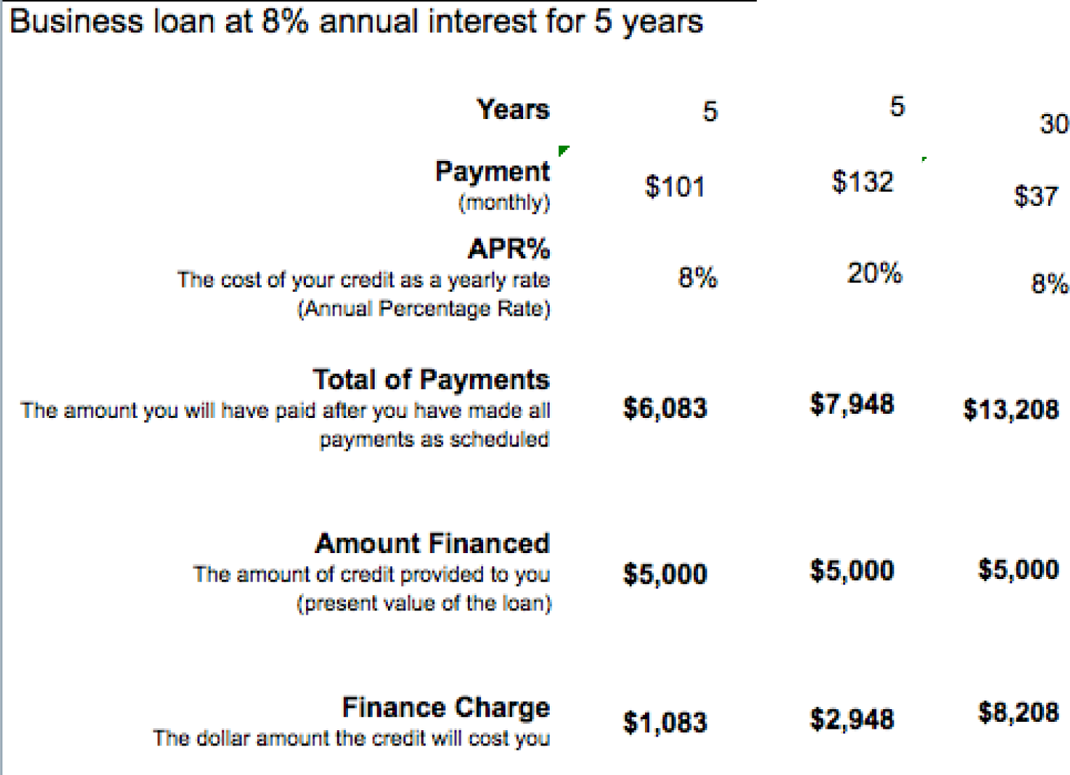
Here the same $5,000 loan is shown under different loan terms. The second loan increases the interest rate to 20%, but leaves all else unchanged from the original. The third loan increases the term of the loan to thirty years but leaves all else unchanged from the original. The lesson here is to borrow at as low an interest rate as possible and for as short a time as possible.
So the bottom line is that you should borrow money for as short a time as possible to avoid large finance charges.
By the way, the situation is even worse with credit card loans because the interest rate on credit cards is so much higher—around 20%. Note how at 20% the finance charge climbs to almost $3,000 over five years. Your goal should be to pay off your credit card in full at the end of each month. If you do not have enough money to do this, then you should try to modify spending habits so that you reach this goal.
The following techniques, found in the Excel section of the software reference, may be useful in completing the assignments for this chapter: Conditional Formatting
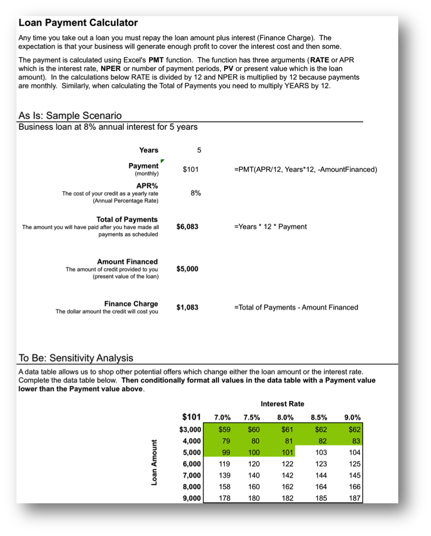
Create a properly formatted spreadsheet that calculates the payments on a business loan.
Many businesses need to take out loans to cover startup costs. This exercise allows you to create a loan payment calculator and perform a sensitivity analysisAn analysis of how the calculation results vary with changes in the initial assumptions. on the terms of the loan.
Setup
Start Excel and properly title your spreadsheet. Because there are so few numbers the assumptions area and the calculations are combined.
Content and Style
Deliverables
Electronic submission: Submit the workbook electronically.
Paper submission:
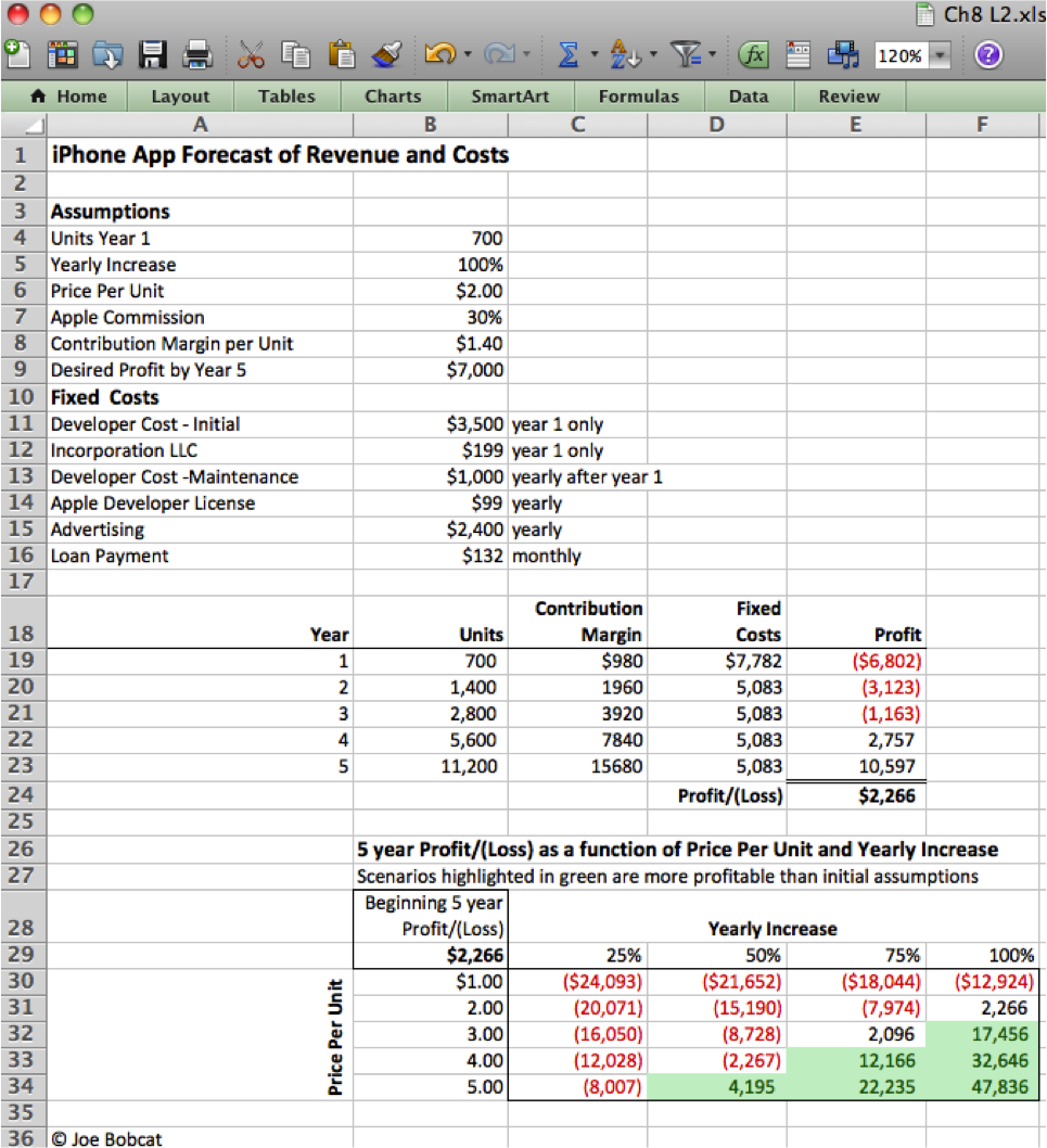
Include loan payments in your previous forecast of revenues and costs.
To make the problem more realistic we bring in loan payments as an additional fixed cost. To help in decision making we conditionally format the sensitivity analysis.
Setup
Open your workbook file from the L2 assignment of the prior chapter, re—save it under a different name, and then modify it to look as below.
Content and Style
Deliverables
Electronic submission: Submit the workbook electronically.
Paper submission:
Add assumptions and columns as necessary to accommodate loan payments.