The aggregate supply and aggregate demand (ASAD) model is presented here. To understand the ASAD model, we need to explain both aggregate demand and aggregate supply and then the determination of prices and output.
The aggregate demand curve tells us the level of expenditure in an economy for a given price level. It has a negative slope: the demand for real gross domestic product (real GDP) decreases when the price level increases. The downward sloping aggregate demand curve does not follow from the microeconomic “law of demand.” As the price level increases, all prices in an economy increase together. The substitution of expensive goods for cheap goods, which underlies the law of demand, does not occur in the aggregate economy.
Instead, the downward sloping demand curve comes from other forces. First, as prices rise, the real value of nominal wealth falls, and this leads to a fall in household spending. Second, as prices rise today relative to future prices, households are induced to postpone consumption. Finally, a higher price level can lead to a higher interest rate through the response of monetary policy. All these factors together imply that higher prices lead to lower overall demand for real GDP.
Aggregate supply is equal to potential output at all prices. Potential output is determined by the available technology, physical capital, and labor force and is unaffected by the price level. Thus the aggregate supply curve is vertical. In contrast to a firm’s supply curve, as the price level increases, all prices in an economy increase. This includes the prices of inputs, such as labor, into the production process. Since no relative prices change when the price level increases, firms are not induced to change the quantity they supply. Thus aggregate supply is vertical.
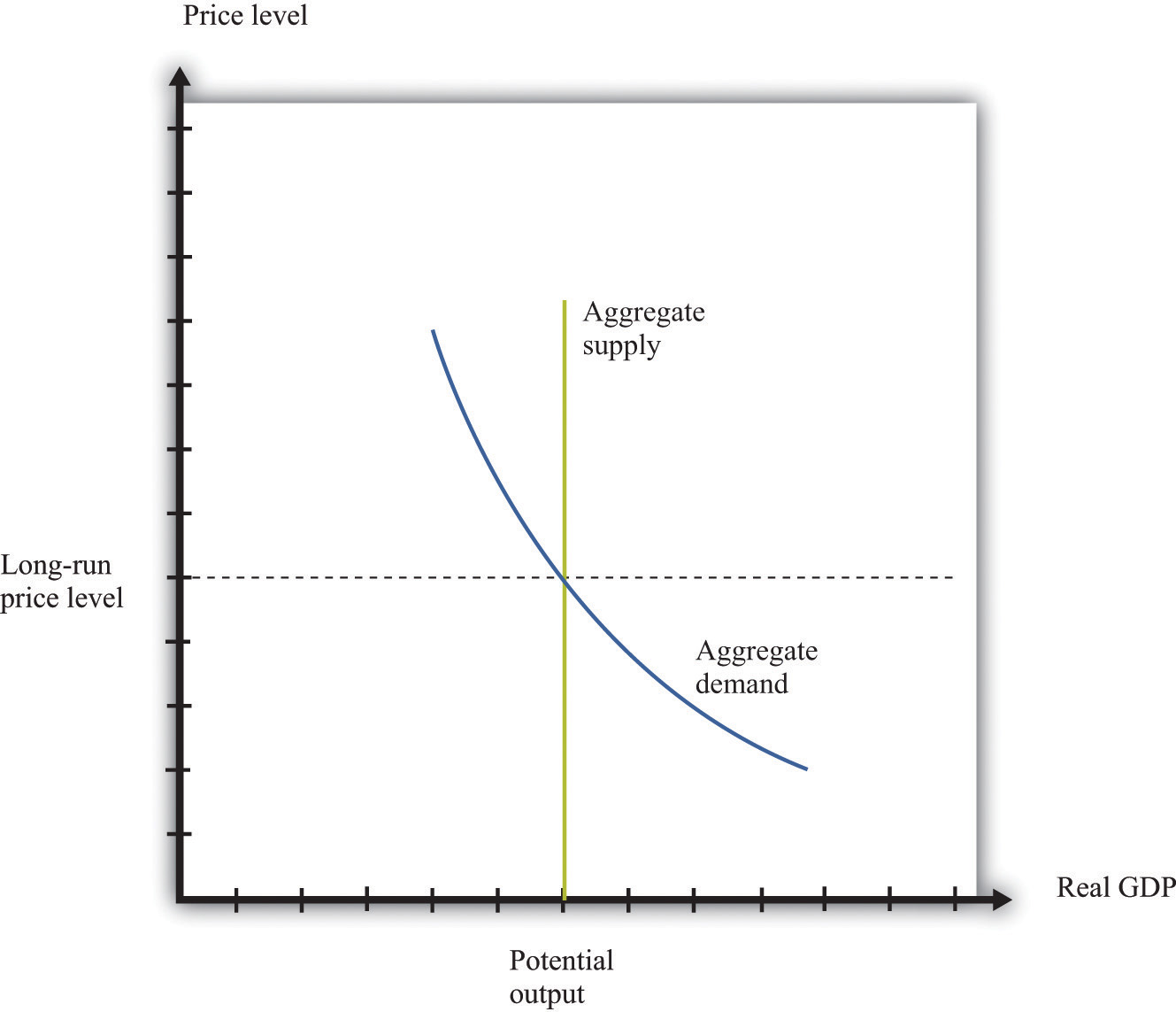
The determination of prices and output depends on the horizon: the long run or the short run. In the long run, real GDP equals potential GDP, and real GDP also equals aggregate expenditure. This means that, in the long run, the price level must be at the point where aggregate demand and aggregate supply meet. This is shown in Figure 16.15 "Aggregate Supply and Aggregate Demand in the Long Run".
Figure 16.15 Aggregate Supply and Aggregate Demand in the Long Run
In the short run, output is determined by aggregate demand at the existing price level. Prices need not be at their long-run equilibrium levels. If they are not, then output will not equal potential output. This is shown in Figure 16.16 "Aggregate Supply and Aggregate Demand in the Short Run".
Figure 16.16 Aggregate Supply and Aggregate Demand in the Short Run
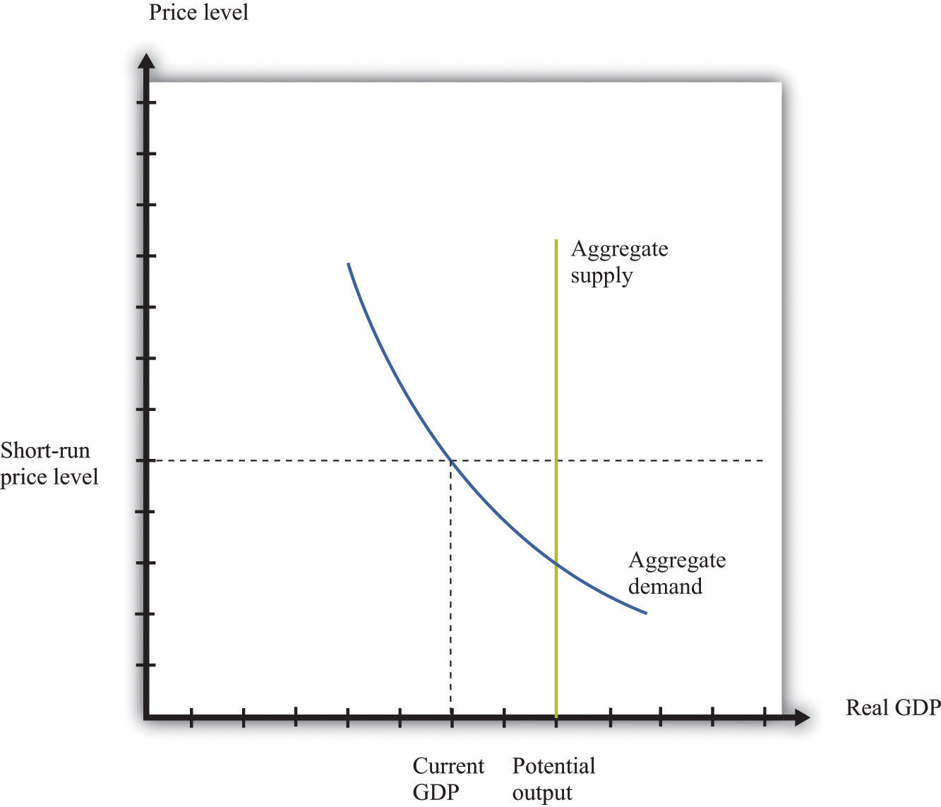
The short-run price level is indicated on the vertical axis. The level of output is determined by aggregate demand at that price level. As prices are greater than the long-run equilibrium level of prices, output is below potential output. The price level adjusts over time to its long-run level, according to the price-adjustment equation.
We do not explicitly use this tool in our chapter presentations. However, the tool can be used to support the discussions in the following chapters.


