The IS-LM model provides another way of looking at the determination of the level of short-run real gross domestic product (real GDP) in the economy. Like the aggregate expenditure model, it takes the price level as fixed. But whereas that model takes the interest rate as exogenous—specifically, a change in the interest rate results in a change in autonomous spending—the IS-LM model treats the interest rate as an endogenous variable.
The basis of the IS-LM model is an analysis of the money market and an analysis of the goods market, which together determine the equilibrium levels of interest rates and output in the economy, given prices. The model finds combinations of interest rates and output (GDP) such that the money market is in equilibrium. This creates the LM curve. The model also finds combinations of interest rates and output such that the goods market is in equilibrium. This creates the IS curve. The equilibrium is the interest rate and output combination that is on both the IS and the LM curves.
The LM curve represents the combinations of the interest rate and income such that money supply and money demand are equal. The demand for money comes from households, firms, and governments that use money as a means of exchange and a store of value. The law of demand holds: as the interest rate increases, the quantity of money demanded decreases because the interest rate represents an opportunity cost of holding money. When interest rates are higher, in other words, money is less effective as a store of value.
Money demand increases when output rises because money also serves as a medium of exchange. When output is larger, people have more income and so want to hold more money for their transactions.
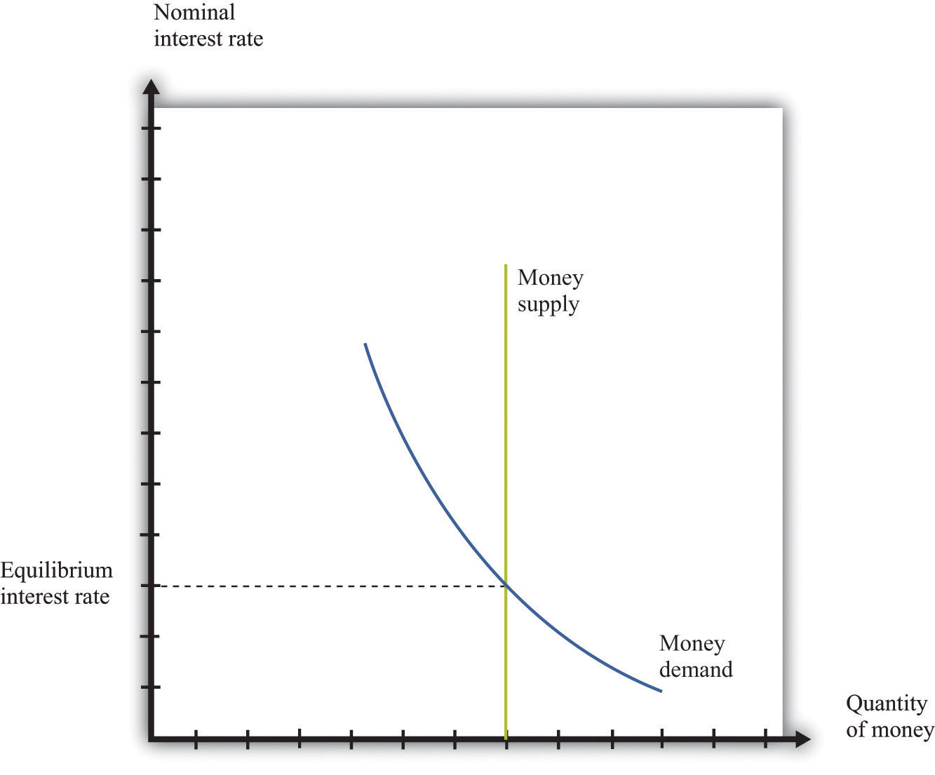
The supply of money is chosen by the monetary authority and is independent of the interest rate. Thus it is drawn as a vertical line. The equilibrium in the money market is shown in Figure 16.17 "Money Market Equilibrium". When the money supply is chosen by the monetary authority, the interest rate is the price that brings the market into equilibrium. Sometimes, in some countries, central banks target the money supply. Alternatively, central banks may choose to target the interest rate. (This was the case we considered in Chapter 10 "Understanding the Fed".) Figure 16.17 "Money Market Equilibrium" applies in either case: if the monetary authority targets the interest rate, then the money market tells us what the level of the money supply must be.
Figure 16.17 Money Market Equilibrium
To trace out the LM curve, we look at what happens to the interest rate when the level of output in the economy changes and the supply of money is held fixed. Figure 16.18 "A Change in Income" shows the money market equilibrium at two different levels of real GDP. At the higher level of income, money demand is shifted to the right; the interest rate increases to ensure that money demand equals money supply. Thus the LM curve is upward sloping: higher real GDP is associated with higher interest rates. At each point along the LM curve, money supply equals money demand.
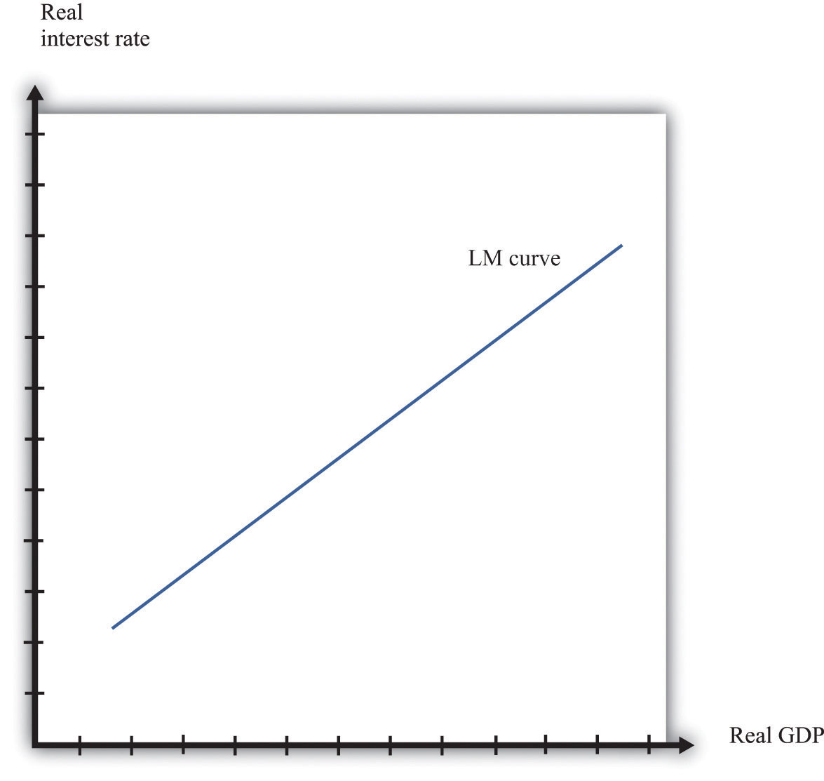
We have not yet been specific about whether we are talking about nominal interest rates or real interest rates. In fact, it is the nominal interest rate that represents the opportunity cost of holding money. When we draw the LM curve, however, we put the real interest rate on the axis, as shown in Figure 16.19 "The LM Curve". The simplest way to think about this is to suppose that we are considering an economy where the inflation rate is zero. In this case, by the Fisher equation, the nominal and real interest rates are the same. In a more complete analysis, we can incorporate inflation by noting that changes in the inflation rate will shift the LM curve. Changes in the money supply also shift the LM curve.
Figure 16.18 A Change in Income
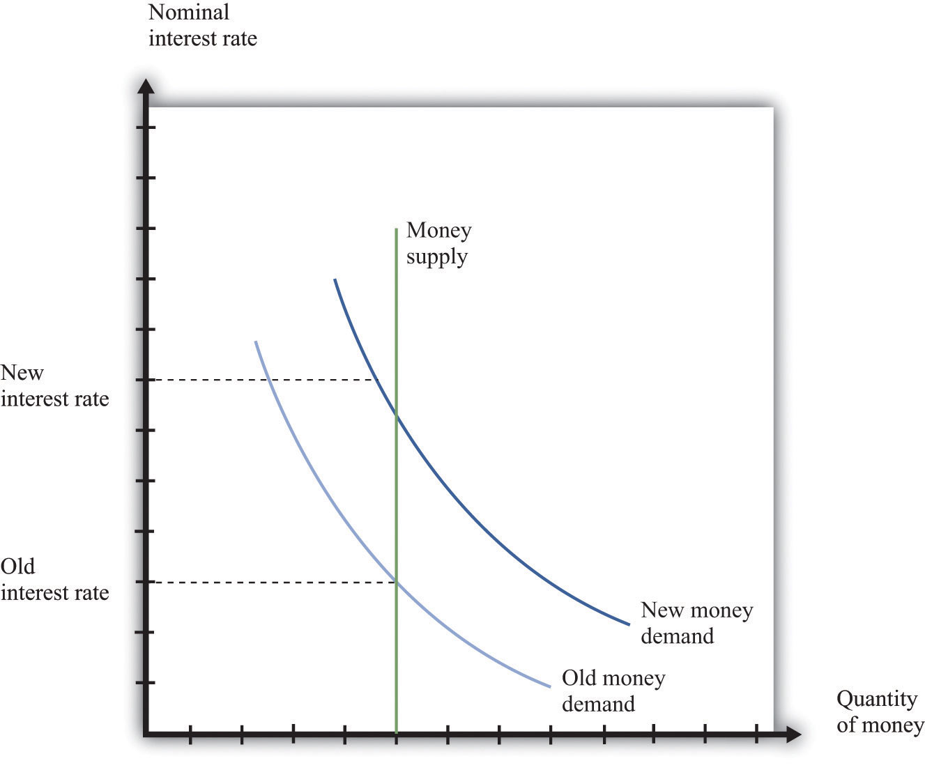
Figure 16.19 The LM Curve
The IS curve relates the level of real GDP and the real interest rate. It incorporates both the dependence of spending on the real interest rate and the fact that, in the short run, real GDP equals spending. The IS curve is shown in Figure 16.18 "A Change in Income". We label the horizontal axis “real GDP” since, in the short run, real GDP is determined by aggregate spending. The IS curve is downward sloping: as the real interest rate increases, the level of spending decreases.
Figure 16.20 The IS Curve
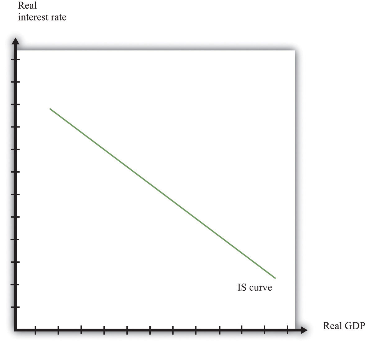
In fact, we derived the IS curve in Chapter 10 "Understanding the Fed". The dependence of spending on real interest rates comes partly from investment. As the real interest rate increases, spending by firms on new capital and spending by households on new housing decreases. Consumption also depends on the real interest rate: spending by households on durable goods decreases as the real interest rate increases.
The connection between spending and real GDP comes from the aggregate expenditure model. Given a particular level of the interest rate, the aggregate expenditure model determines the level of real GDP. Now suppose the interest rate increases. This reduces those components of spending that depend on the interest rate. In the aggregate expenditure framework, this is a reduction in autonomous spending. The equilibrium level of output decreases. Thus the IS curve slopes downwards: higher interest rates are associated with lower real GDP.
Combining the discussion of the LM and the IS curves will generate equilibrium levels of interest rates and output. Note that both relationships are combinations of interest rates and output. Solving these two equations jointly determines the equilibrium. This is shown graphically in Figure 16.21. This just combines the LM curve from Figure 16.19 "The LM Curve" and the IS curve from Figure 16.20 "The IS Curve". The crossing of these two curves is the combination of the interest rate and real GDP, denoted (r*,Y*), such that both the money market and the goods market are in equilibrium.
Figure 16.21
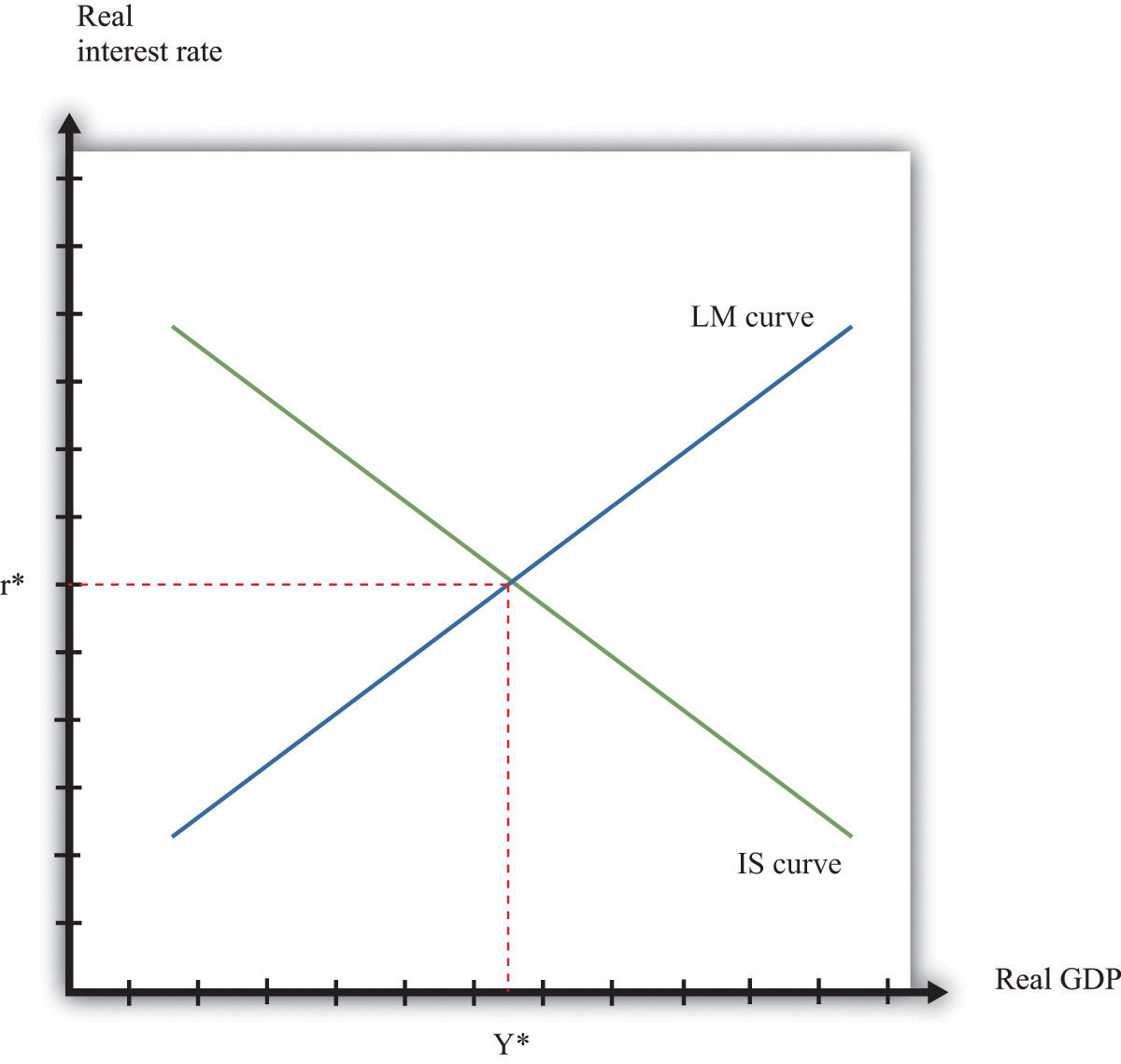
Equilibrium in the IS-LM Model.
Comparative statics results for this model illustrate how changes in exogenous factors influence the equilibrium levels of interest rates and output. For this model, there are two key exogenous factors: the level of autonomous spending (excluding any spending affected by interest rates) and the real money supply. We can study how changes in these factors influence the equilibrium levels of output and interest rates both graphically and algebraically.
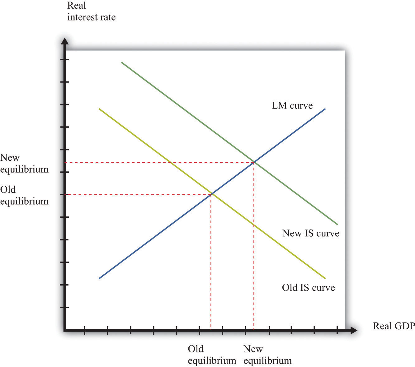
Variations in the level of autonomous spending will lead to a shift in the IS curve, as shown in Figure 16.22 "A Shift in the IS Curve". If autonomous spending increases, then the IS curve shifts out. The output level of the economy will increase. Interest rates rise as we move along the LM curve, ensuring money market equilibrium. One source of variations in autonomous spending is fiscal policy. Autonomous spending includes government spending (G). Thus an increase in G leads to an increase in output and interest rates as shown in Figure 16.22 "A Shift in the IS Curve".
Figure 16.22 A Shift in the IS Curve
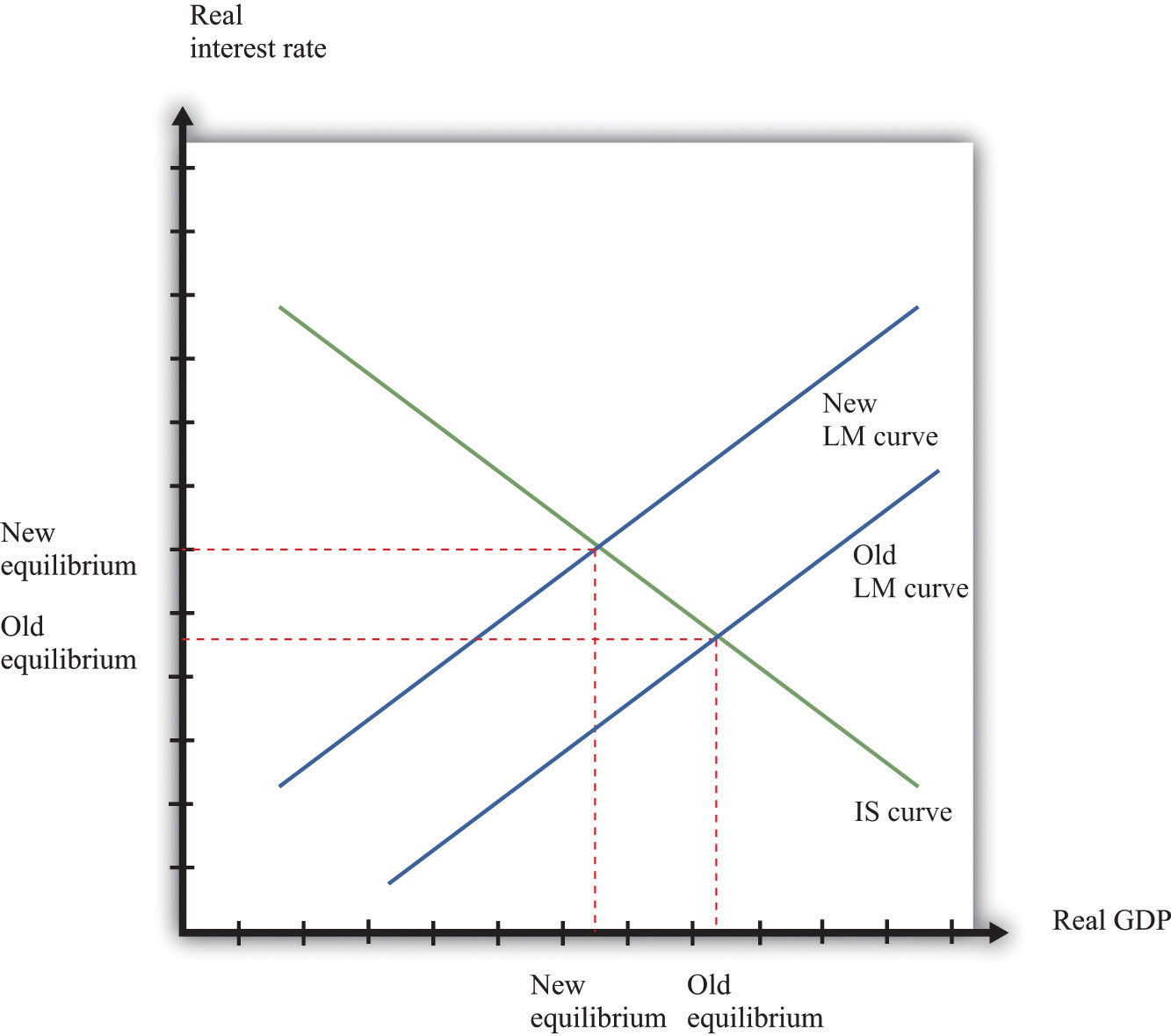
Variations in the real money supply shift the LM curve, as shown in Figure 16.23 "A Shift in the LM Curve". If the money supply decreases, then the LM curve shifts in. This leads to a higher real interest rate and lower output as the LM curve shifts along the fixed IS curve.
Figure 16.23 A Shift in the LM Curve
We can represent the LM and IS curves algebraically.
Let L(Y,r) represent real money demand at a level of real GDP of Y and a real interest rate of r. (When we say “real” money demand, we mean that, as usual, we have deflated by the price level.) For simplicity, suppose that the inflation rate is zero, so the real interest rate is the opportunity cost of holding money.If we wanted to include inflation in our analysis, we could write the real demand for money as L(Y, r + π), where π is the inflation rate. Assume that real money demand takes a particular form:
L(Y,r) = L0 + L1Y – L2r.In this equation, L0, L1, and L2 are all positive constants. Real money demand is increasing in income and decreasing in the interest rate. Letting M/P be the real stock of money in the economy, then money market equilibrium requires
M/P = L0 + L1Y – L2r.Given a level of real GDP and the real stock of money, this equation can be used to solve for the interest rate such that money supply and money demand are equal. This is given by
r = (1/L2) [L0 + L1Y – M/P].From this equation we learn that an increase in the real stock of money lowers the interest rate, given the level of real GDP. Further, an increase in the level of real GDP increases the interest rate, given the stock of money. This is another way of saying that the LM curve is upward sloping.
Recall the two equations from the aggregate expenditure model:
Y = Eand
E = E0(r) + βY.Here we have shown explicitly that the level of autonomous spending depends on the real interest rate r.
We can solve the two equations to find the values of E and Y that are consistent with both equations. We find
Given a level of the real interest rate, we solve for the level of autonomous spending (using the dependence of consumption and investment on the real interest rate) and then use this equation to find the level of output.
Here is an example. Suppose that
C = 100 + 0.6Y, I = 400 − 5r, G = 300,and
NX = 200 − 0.1Y,where C is consumption, I is investment, G is government purchases, and NX is net exports. First group the components of spending as follows:
C + I + G + NX = (100 + 400 − 5r + 300 + 200) + (0.6Y − 0.1Y)Adding together the first group of terms, we find autonomous spending:
E0 = 100 + 400 + 300 + 200 − 5r = 1000 − 5r.Adding the coefficients on the income terms, we find the marginal propensity to spend:
β = 0.6 − 0.1 = 0.5.Using β = 0.5, we calculate the multiplier:
We then calculate real GDP, given the real interest rate:
Y = 2 × (1000 − 5r) = 2000 − 10r.Combining the discussion of the LM and the IS curves will generate equilibrium levels of interest rates and output. Note that both relationships are combinations of interest rates and output. Solving these two equations jointly determines the equilibrium.
Algebraically, we have an equation for the LM curve:
r = (1/L2) [L0 + L1Y – M/P].And we have an equation for the IS curve:
Y = mE0(r),where we let m = (1/(1 – β)) denote the multiplier. If we assume that the dependence of spending in the interest rate is linear, so that E0(r) = e0 – e1r, then the equation for the IS curve is
Y = m (e0-e1r),To solve the IS and LM curves simultaneously, we substitute Y from the IS curve into the LM curve to get
r = (1/L2) [L0 + L1 m(e0-e1r) – M/P].Solving this for r we get
r = Ar – BrM/P.where both Ar and Br are constants, with Ar = (L0 + L1me0)/(L1me1 + L2) and Br = 1/(L1me1 + L2). This equation gives us the equilibrium level of the real interest rate given the level of autonomous spending, summarized by e0, and the real stock of money, summarized by M/P.
To find the equilibrium level of output, we substitute this equation for r back into the equation for the IS curve. This gives us
Y = Ay + By(M/P),where both Ay and By are constants, with Ay = m(e0 – e1Ar) and By = me1Br. This equation gives us the equilibrium level of output given the level of autonomous spending, summarized by e0, and the real stock of money, summarized by M/P.
Algebraically, we can use the equations to determine the magnitude of the responses of interest rates and output to exogenous changes. An increase in the autonomous spending, e0, will increase both Ar and Ay, implying that both the interest rate and output increase.To see that Ay increases with e0 requires a bit more algebra. An increase in the real money stock will reduce interest rates by Br and increase output by By. A key part of monetary policy is the sensitivity of spending to the interest rate, given by e1. The more sensitive is spending to the interest rate, the larger is e1 and therefore the larger is By.
We do not explicitly use this tool in our chapter presentations. However, the tool can be used to support the discussions in the following chapters.

