How many pizzas will people eat this year? How many doctor visits will people make? How many houses will people buy?
Each good or service has its own special characteristics that determine the quantity people are willing and able to consume. One is the price of the good or service itself. Other independent variables that are important determinants of demand include consumer preferences, prices of related goods and services, income, demographic characteristics such as population size, and buyer expectations. The number of pizzas people will purchase, for example, depends very much on how much they like pizza. It also depends on the prices for alternatives such as hamburgers or spaghetti. The number of doctor visits is likely to vary with income—people with higher incomes are likely to see a doctor more often than people with lower incomes. The demands for pizza, for doctor visits, and for housing are certainly affected by the age distribution of the population and its size.
While different variables play different roles in influencing the demands for different goods and services, economists pay special attention to one: the price of the good or service. Given the values of all the other variables that affect demand, a higher price tends to reduce the quantity people demand, and a lower price tends to increase it. A medium pizza typically sells for $5 to $10. Suppose the price were $30. Chances are, you would buy fewer pizzas at that price than you do now. Suppose pizzas typically sold for $2 each. At that price, people would be likely to buy more pizzas than they do now.
We will discuss first how price affects the quantity demanded of a good or service and then how other variables affect demand.
Because people will purchase different quantities of a good or service at different prices, economists must be careful when speaking of the “demand” for something. They have therefore developed some specific terms for expressing the general concept of demand.
The quantity demandedThe quantity buyers are willing and able to buy of a good or service at a particular price during a particular period, all other things unchanged. of a good or service is the quantity buyers are willing and able to buy at a particular price during a particular period, all other things unchanged. (As we learned, we can substitute the Latin phrase “ceteris paribus” for “all other things unchanged.”) Suppose, for example, that 100,000 movie tickets are sold each month in a particular town at a price of $8 per ticket. That quantity—100,000—is the quantity of movie admissions demanded per month at a price of $8. If the price were $12, we would expect the quantity demanded to be less. If it were $4, we would expect the quantity demanded to be greater. The quantity demanded at each price would be different if other things that might affect it, such as the population of the town, were to change. That is why we add the qualifier that other things have not changed to the definition of quantity demanded.
A demand scheduleA table that shows the quantities of a good or service demanded at different prices during a particular period, all other things unchanged. is a table that shows the quantities of a good or service demanded at different prices during a particular period, all other things unchanged. To introduce the concept of a demand schedule, let us consider the demand for coffee in the United States. We will ignore differences among types of coffee beans and roasts, and speak simply of coffee. The table in Figure 3.1 "A Demand Schedule and a Demand Curve" shows quantities of coffee that will be demanded each month at prices ranging from $9 to $4 per pound; the table is a demand schedule. We see that the higher the price, the lower the quantity demanded.
Figure 3.1 A Demand Schedule and a Demand Curve
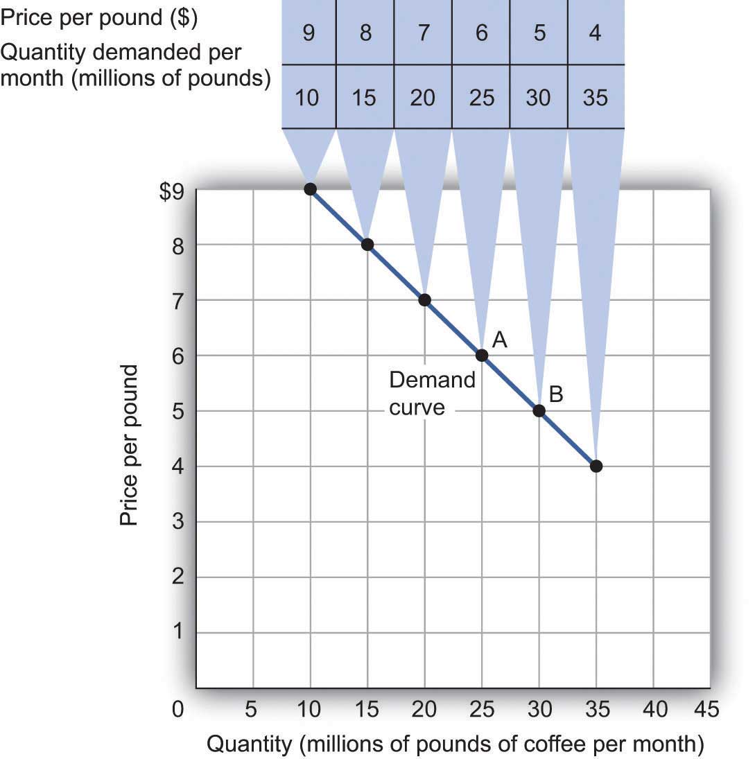
The table is a demand schedule; it shows quantities of coffee demanded per month in the United States at particular prices, all other things unchanged. These data are then plotted on the demand curve. At point A on the curve, 25 million pounds of coffee per month are demanded at a price of $6 per pound. At point B, 30 million pounds of coffee per month are demanded at a price of $5 per pound.
The information given in a demand schedule can be presented with a demand curveA graphical representation of a demand schedule., which is a graphical representation of a demand schedule. A demand curve thus shows the relationship between the price and quantity demanded of a good or service during a particular period, all other things unchanged. The demand curve in Figure 3.1 "A Demand Schedule and a Demand Curve" shows the prices and quantities of coffee demanded that are given in the demand schedule. At point A, for example, we see that 25 million pounds of coffee per month are demanded at a price of $6 per pound. By convention, economists graph price on the vertical axis and quantity on the horizontal axis.
Price alone does not determine the quantity of coffee or any other good that people buy. To isolate the effect of changes in price on the quantity of a good or service demanded, however, we show the quantity demanded at each price, assuming that those other variables remain unchanged. We do the same thing in drawing a graph of the relationship between any two variables; we assume that the values of other variables that may affect the variables shown in the graph (such as income or population) remain unchanged for the period under consideration.
A change in price, with no change in any of the other variables that affect demand, results in a movement along the demand curve. For example, if the price of coffee falls from $6 to $5 per pound, consumption rises from 25 million pounds to 30 million pounds per month. That is a movement from point A to point B along the demand curve in Figure 3.1 "A Demand Schedule and a Demand Curve". A movement along a demand curve that results from a change in price is called a change in quantity demandedA movement along a demand curve that results from a change in price.. Note that a change in quantity demanded is not a change or shift in the demand curve; it is a movement along the demand curve.
The negative slope of the demand curve in Figure 3.1 "A Demand Schedule and a Demand Curve" suggests a key behavioral relationship in economics. All other things unchanged, the law of demandFor virtually all goods and services, a higher price leads to a reduction in quantity demanded and a lower price leads to an increase in quantity demanded. holds that, for virtually all goods and services, a higher price leads to a reduction in quantity demanded and a lower price leads to an increase in quantity demanded.
The law of demand is called a law because the results of countless studies are consistent with it. Undoubtedly, you have observed one manifestation of the law. When a store finds itself with an overstock of some item, such as running shoes or tomatoes, and needs to sell these items quickly, what does it do? It typically has a sale, expecting that a lower price will increase the quantity demanded. In general, we expect the law of demand to hold. Given the values of other variables that influence demand, a higher price reduces the quantity demanded. A lower price increases the quantity demanded. Demand curves, in short, slope downward.
Of course, price alone does not determine the quantity of a good or service that people consume. Coffee consumption, for example, will be affected by such variables as income and population. Preferences also play a role. The story at the beginning of the chapter illustrates how Starbucks “turned people on” to coffee. We also expect other prices to affect coffee consumption. People often eat doughnuts or bagels with their coffee, so a reduction in the price of doughnuts or bagels might induce people to drink more coffee. An alternative to coffee is tea, so a reduction in the price of tea might result in the consumption of more tea and less coffee. Thus, a change in any one of the variables held constant in constructing a demand schedule will change the quantities demanded at each price. The result will be a shift in the entire demand curve rather than a movement along the demand curve. A shift in a demand curve is called a change in demandA shift in a demand curve..
Suppose, for example, that something happens to increase the quantity of coffee demanded at each price. Several events could produce such a change: an increase in incomes, an increase in population, or an increase in the price of tea would each be likely to increase the quantity of coffee demanded at each price. Any such change produces a new demand schedule. Figure 3.2 "An Increase in Demand" shows such a change in the demand schedule for coffee. We see that the quantity of coffee demanded per month is greater at each price than before. We show that graphically as a shift in the demand curve. The original curve, labeled D1, shifts to the right to D2. At a price of $6 per pound, for example, the quantity demanded rises from 25 million pounds per month (point A) to 35 million pounds per month (point A′).
Figure 3.2 An Increase in Demand
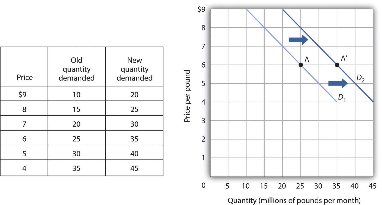
An increase in the quantity of a good or service demanded at each price is shown as an increase in demand. Here, the original demand curve D1 shifts to D2. Point A on D1 corresponds to a price of $6 per pound and a quantity demanded of 25 million pounds of coffee per month. On the new demand curve D2, the quantity demanded at this price rises to 35 million pounds of coffee per month (point A′).
Just as demand can increase, it can decrease. In the case of coffee, demand might fall as a result of events such as a reduction in population, a reduction in the price of tea, or a change in preferences. For example, a definitive finding that the caffeine in coffee contributes to heart disease, which is currently being debated in the scientific community, could change preferences and reduce the demand for coffee.
A reduction in the demand for coffee is illustrated in Figure 3.3 "A Reduction in Demand". The demand schedule shows that less coffee is demanded at each price than in Figure 3.1 "A Demand Schedule and a Demand Curve". The result is a shift in demand from the original curve D1 to D3. The quantity of coffee demanded at a price of $6 per pound falls from 25 million pounds per month (point A) to 15 million pounds per month (point A″). Note, again, that a change in quantity demanded, ceteris paribus, refers to a movement along the demand curve, while a change in demand refers to a shift in the demand curve.
Figure 3.3 A Reduction in Demand
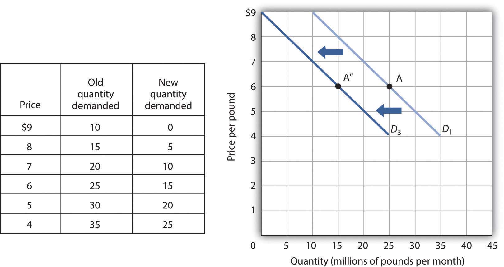
A reduction in demand occurs when the quantities of a good or service demanded fall at each price. Here, the demand schedule shows a lower quantity of coffee demanded at each price than we had in Figure 3.1 "A Demand Schedule and a Demand Curve". The reduction shifts the demand curve for coffee to D3 from D1. The quantity demanded at a price of $6 per pound, for example, falls from 25 million pounds per month (point A) to 15 million pounds of coffee per month (point A″).
A variable that can change the quantity of a good or service demanded at each price is called a demand shifterA variable that can change the quantity of a good or service demanded at each price.. When these other variables change, the all-other-things-unchanged conditions behind the original demand curve no longer hold. Although different goods and services will have different demand shifters, the demand shifters are likely to include (1) consumer preferences, (2) the prices of related goods and services, (3) income, (4) demographic characteristics, and (5) buyer expectations. Next we look at each of these.
Changes in preferences of buyers can have important consequences for demand. We have already seen how Starbucks supposedly increased the demand for coffee. Another example is reduced demand for cigarettes caused by concern about the effect of smoking on health. A change in preferences that makes one good or service more popular will shift the demand curve to the right. A change that makes it less popular will shift the demand curve to the left.
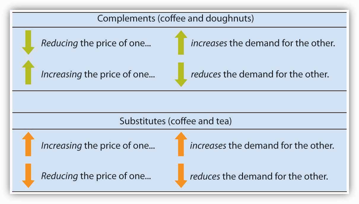
Suppose the price of doughnuts were to fall. Many people who drink coffee enjoy dunking doughnuts in their coffee; the lower price of doughnuts might therefore increase the demand for coffee, shifting the demand curve for coffee to the right. A lower price for tea, however, would be likely to reduce coffee demand, shifting the demand curve for coffee to the left.
In general, if a reduction in the price of one good increases the demand for another, the two goods are called complementsTwo goods for which an increase in price of one reduces the demand for the other.. If a reduction in the price of one good reduces the demand for another, the two goods are called substitutesTwo goods for which an increase in price of one increases the demand for the other.. These definitions hold in reverse as well: two goods are complements if an increase in the price of one reduces the demand for the other, and they are substitutes if an increase in the price of one increases the demand for the other. Doughnuts and coffee are complements; tea and coffee are substitutes.
Complementary goods are goods used in conjunction with one another. Tennis rackets and tennis balls, eggs and bacon, and stationery and postage stamps are complementary goods. Substitute goods are goods used instead of one another. iPODs, for example, are likely to be substitutes for CD players. Breakfast cereal is a substitute for eggs. A file attachment to an e-mail is a substitute for both a fax machine and postage stamps.
As incomes rise, people increase their consumption of many goods and services, and as incomes fall, their consumption of these goods and services falls. For example, an increase in income is likely to raise the demand for gasoline, ski trips, new cars, and jewelry. There are, however, goods and services for which consumption falls as income rises—and rises as income falls. As incomes rise, for example, people tend to consume more fresh fruit but less canned fruit.
A good for which demand increases when income increases is called a normal goodA good for which demand increases when income increases.. A good for which demand decreases when income increases is called an inferior goodA good for which demand decreases when income increases.. An increase in income shifts the demand curve for fresh fruit (a normal good) to the right; it shifts the demand curve for canned fruit (an inferior good) to the left.
The number of buyers affects the total quantity of a good or service that will be bought; in general, the greater the population, the greater the demand. Other demographic characteristics can affect demand as well. As the share of the population over age 65 increases, the demand for medical services, ocean cruises, and motor homes increases. The birth rate in the United States fell sharply between 1955 and 1975 but has gradually increased since then. That increase has raised the demand for such things as infant supplies, elementary school teachers, soccer coaches, in-line skates, and college education. Demand can thus shift as a result of changes in both the number and characteristics of buyers.
The consumption of goods that can be easily stored, or whose consumption can be postponed, is strongly affected by buyer expectations. The expectation of newer TV technologies, such as high-definition TV, could slow down sales of regular TVs. If people expect gasoline prices to rise tomorrow, they will fill up their tanks today to try to beat the price increase. The same will be true for goods such as automobiles and washing machines: an expectation of higher prices in the future will lead to more purchases today. If the price of a good is expected to fall, however, people are likely to reduce their purchases today and await tomorrow’s lower prices. The expectation that computer prices will fall, for example, can reduce current demand.
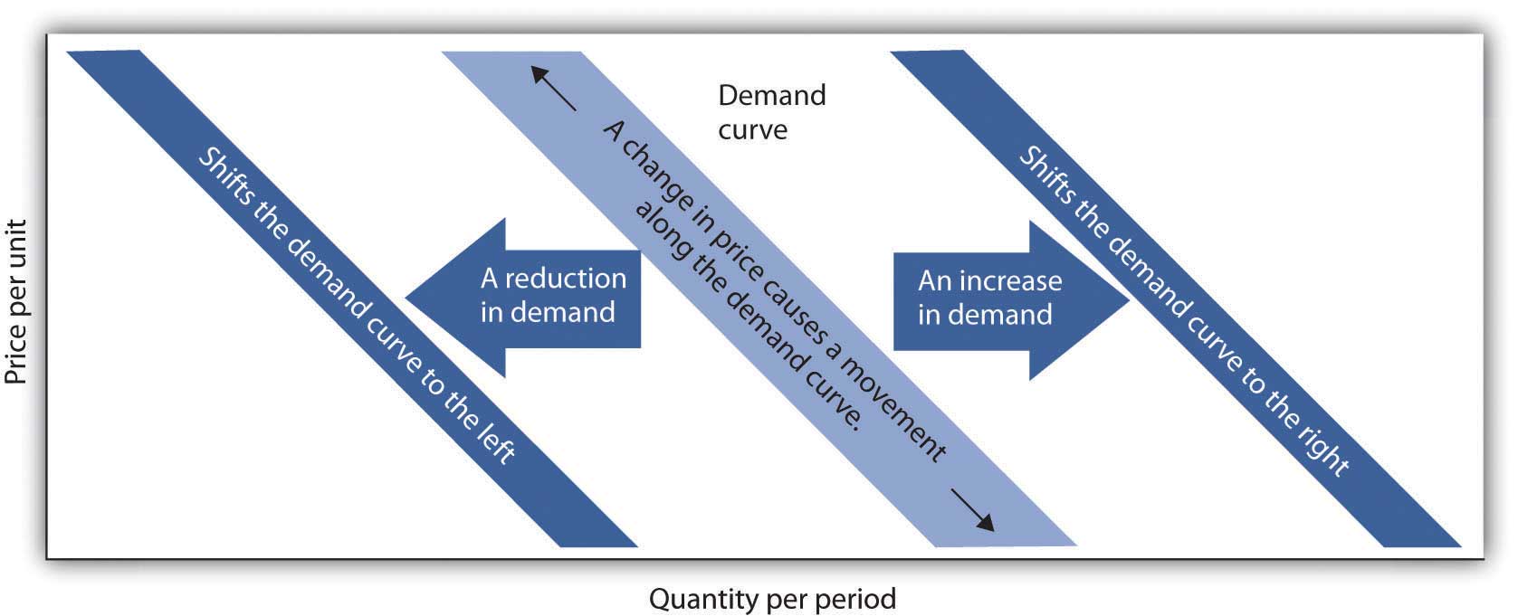
It is crucial to distinguish between a change in quantity demanded, which is a movement along the demand curve caused by a change in price, and a change in demand, which implies a shift of the demand curve itself. A change in demand is caused by a change in a demand shifter. An increase in demand is a shift of the demand curve to the right. A decrease in demand is a shift in the demand curve to the left. This drawing of a demand curve highlights the difference.
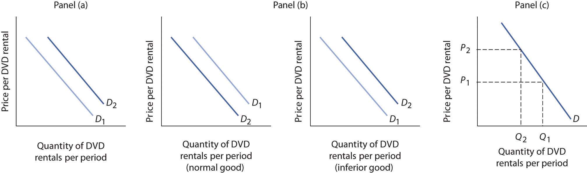
All other things unchanged, what happens to the demand curve for DVD rentals if there is (a) an increase in the price of movie theater tickets, (b) a decrease in family income, or (c) an increase in the price of DVD rentals? In answering this and other “Try It!” problems in this chapter, draw and carefully label a set of axes. On the horizontal axis of your graph, show the quantity of DVD rentals. It is necessary to specify the time period to which your quantity pertains (e.g., “per period,” “per week,” or “per year”). On the vertical axis show the price per DVD rental. Since you do not have specific data on prices and quantities demanded, make a “free-hand” drawing of the curve or curves you are asked to examine. Focus on the general shape and position of the curve(s) before and after events occur. Draw new curve(s) to show what happens in each of the circumstances given. The curves could shift to the left or to the right, or stay where they are.
Unless you attend a “virtual” campus, chances are you have engaged in more than one conversation about how hard it is to find a place to park on campus. Indeed, according to Clark Kerr, a former president of the University of California system, a university is best understood as a group of people “held together by a common grievance over parking.”
Clearly, the demand for campus parking spaces has grown substantially over the past few decades. In surveys conducted by Daniel Kenney, Ricardo Dumont, and Ginger Kenney, who work for the campus design company Sasaki and Associates, it was found that 7 out of 10 students own their own cars. They have interviewed “many students who confessed to driving from their dormitories to classes that were a five-minute walk away,” and they argue that the deterioration of college environments is largely attributable to the increased use of cars on campus and that colleges could better service their missions by not adding more parking spaces.
Since few universities charge enough for parking to even cover the cost of building and maintaining parking lots, the rest is paid for by all students as part of tuition. Their research shows that “for every 1,000 parking spaces, the median institution loses almost $400,000 a year for surface parking, and more than $1,200,000 for structural parking.” Fear of a backlash from students and their parents, as well as from faculty and staff, seems to explain why campus administrators do not simply raise the price of parking on campus.
While Kenney and his colleagues do advocate raising parking fees, if not all at once then over time, they also suggest some subtler, and perhaps politically more palatable, measures—in particular, shifting the demand for parking spaces to the left by lowering the prices of substitutes.
Two examples they noted were at the University of Washington and the University of Colorado at Boulder. At the University of Washington, car poolers may park for free. This innovation has reduced purchases of single-occupancy parking permits by 32% over a decade. According to University of Washington assistant director of transportation services Peter Dewey, “Without vigorously managing our parking and providing commuter alternatives, the university would have been faced with adding approximately 3,600 parking spaces, at a cost of over $100 million…The university has created opportunities to make capital investments in buildings supporting education instead of structures for cars.” At the University of Colorado, free public transit has increased use of buses and light rail from 300,000 to 2 million trips per year over the last decade. The increased use of mass transit has allowed the university to avoid constructing nearly 2,000 parking spaces, which has saved about $3.6 million annually.
Sources: Daniel R. Kenney, “How to Solve Campus Parking Problems Without Adding More Parking,” The Chronicle of Higher Education, March 26, 2004, Section B, pp. B22-B23.
Since going to the movies is a substitute for watching a DVD at home, an increase in the price of going to the movies should cause more people to switch from going to the movies to staying at home and renting DVDs. Thus, the demand curve for DVD rentals will shift to the right when the price of movie theater tickets increases [Panel (a)].
A decrease in family income will cause the demand curve to shift to the left if DVD rentals are a normal good but to the right if DVD rentals are an inferior good. The latter may be the case for some families, since staying at home and watching DVDs is a cheaper form of entertainment than taking the family to the movies. For most others, however, DVD rentals are probably a normal good [Panel (b)].
An increase in the price of DVD rentals does not shift the demand curve for DVD rentals at all; rather, an increase in price, say from P1 to P2, is a movement upward to the left along the demand curve. At a higher price, people will rent fewer DVDs, say Q2 instead of Q1, ceteris paribus [Panel (c)].