How important is economic growth? The best way to answer that question is to imagine life without growth—to imagine that we did not have the gains growth brings.
For starters, divide your family’s current income by six and imagine what your life would be like. Think about the kind of housing your family could afford, the size of your entertainment budget, whether you could still attend school. That will give you an idea of life a century ago in the United States, when average household incomes, adjusted for inflation, were about one-sixth what they are today. People had far smaller homes, they rarely had electricity in their homes, and only a tiny percentage of the population could even consider a college education.
To get a more recent perspective, consider how growth has changed living standards over the past half century or so. In 1950, the United States was the world’s richest nation. But if households were rich then, subsequent economic growth has made them far richer. Average per capita real income has tripled since then. Indeed, the average household income in 1950, which must have seemed lofty then, was below what we now define as the poverty line for a household of four, even after adjusting for inflation. Economic growth during the last 60-plus years has dramatically boosted our standard of living—and our standard of what it takes to get by.
One gauge of rising living standards is housing. A half century ago, most families did not own homes. Today, about two-thirds do. Those homes have gotten a lot bigger: new homes built today are more than twice the size of new homes built 50 years ago. Some household appliances, such as telephones or washing machines, that we now consider basic, were luxuries a half century ago. In 1950, less than two-thirds of housing units had complete plumbing facilities. Today, over 99% do.
Economic growth has brought gains in other areas as well. For one thing, we are able to afford more schooling. In 1950, the median number of years of school completed by adults age 25 or over was 6.8. Today, about 87% have completed 12 years of schooling and about 30% have completed 4 years of college. We also live longer. A baby born in 1950 had a life expectancy of 68 years. A baby born in 2008 had an expected life of nearly 10 years longer.
Of course, while economic growth can improve our material well-being, it is no panacea. Americans today worry about the level of violence in society, environmental degradation, and what seems to be a loss of basic values. But while it is easy to be dismayed about many challenges of modern life, we can surely be grateful for our material wealth. Our affluence gives us the opportunity to grapple with some of our most difficult problems and to enjoy a range of choices that people only a few decades ago could not have imagined.
We learned a great deal about economic growth in the context of the production possibilities curve. Our purpose in this chapter is to relate the concept of economic growth to the model of aggregate demand and aggregate supply that we developed in the previous chapter and will use throughout our exploration of macroeconomics. We will review the forces that determine a nation’s economic growth rate and examine the prospects for growth in the future. We begin by looking at the significance of growth to the overall well-being of society.
To demonstrate the impact of economic growth on living standards of a nation, we must start with a clear definition of economic growth and then study its impact over time. We will also see how population growth affects the relationship between economic growth and the standard of living an economy is able to achieve.
Economic growth is a long-run process that occurs as an economy’s potential output increases. Changes in real GDP from quarter to quarter or even from year to year are short-run fluctuations that occur as aggregate demand and short-run aggregate supply change. Regardless of media reports stating that the economy grew at a certain rate in the last quarter or that it is expected to grow at a particular rate during the next year, short-run changes in real GDP say little about economic growth. In the long run, economic activity moves toward its level of potential output. Increases in potential constitute economic growth.
Earlier we defined economic growth as the process through which an economy achieves an outward shift in its production possibilities curve. How does a shift in the production possibilities curve relate to a change in potential output? To produce its potential level of output, an economy must operate on its production possibilities curve. An increase in potential output thus implies an outward shift in the production possibilities curve. In the framework of the macroeconomic model of aggregate demand and aggregate supply, we show economic growth as a shift to the right in the long-run aggregate supply curve.
There are three key points about economic growth to keep in mind:
Figure 8.1 "A Century of Economic Growth" shows the record of economic growth for the U.S. economy over the past century. The graph shows annual levels of actual real GDP and of potential output. We see that the economy has experienced dramatic growth over the past century; potential output has soared nearly 20-fold. The figure also reminds us of a central theme of our analysis of macroeconomics: real GDP fluctuates about potential output. Real GDP sagged well below its potential (initially more than 40% below and then remaining at about 20% below for most of the decade) during the Great Depression of the 1930s and rose well above its potential (about 30% above) as the nation mobilized its resources to fight World War II. With the exception of these two periods, real GDP has remained fairly close to the economy’s potential output. In the recession of 1981, real GDP was about 6.5% below its potential, and during the recession that began at the end of 2007, real GDP fell nearly 8% below its potential. In 2011, the economy was still about 6.8% below its potential. Nonetheless, since 1950, the actual level of real GDP has deviated from potential output by an average of less than 2%.
Figure 8.1 A Century of Economic Growth
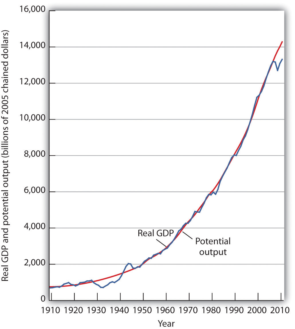
At the start of the 21st century, the level of potential output reached a level nearly 20 times its level a century earlier. Over the years, actual real GDP fluctuated about a rising level of potential output.
Sources: 1910–1949 data from Christina D. Romer, “World War I and the Postwar Depression: A Reinterpretation Based on Alternative Estimates of GNP,” Journal of Monetary Economics 22 (1988): 91–115; data for 1950–2010 from Congressional Budget Office, The Budget and Economic Outlook: An Update, August 2011 and from Bureau of Economic Analysis, NIPA Table 1.1.6.
We urge you to take some time with Figure 8.1 "A Century of Economic Growth". Over the course of the last century, it is economic growth that has taken center stage. Certainly, the fluctuations about potential output have been important. The recessionary gaps—periods when real GDP slipped below its potential—were often wrenching experiences in which millions of people endured great hardship. The inflationary gaps—periods when real GDP rose above its potential level—often produced dramatic increases in price levels. Those fluctuations mattered. It was the unemployment and/or the inflation that came with them that made headlines. But it was the quiet process of economic growth that pushed living standards ever higher. We must understand growth if we are to understand how we got where we are, and where we are likely to be going during the 21st century.
Figure 8.2 "Cyclical Change Versus Growth" tells us why we use changes in potential output, rather than actual real GDP, as our measure of economic growth. Actual values of real GDP are affected not just by changes in the potential level of output, but also by the cyclical fluctuations about that level of output.
Given our definition of economic growth, we would say that the hypothetical economy depicted in Figure 8.2 "Cyclical Change Versus Growth" grew at a 2.5% annual rate throughout the period. If we used actual values of real GDP, however, we would obtain quite different interpretations. Consider, for example, the first decade of this period: it began with a real GDP of $900 billion and a recessionary gap, and it ended in year 10 with a real GDP of $1,408 billion and an inflationary gap. If we record growth as the annual rate of change between these levels, we find an annual rate of growth of 4.6%—a rather impressive performance.
Figure 8.2 Cyclical Change Versus Growth
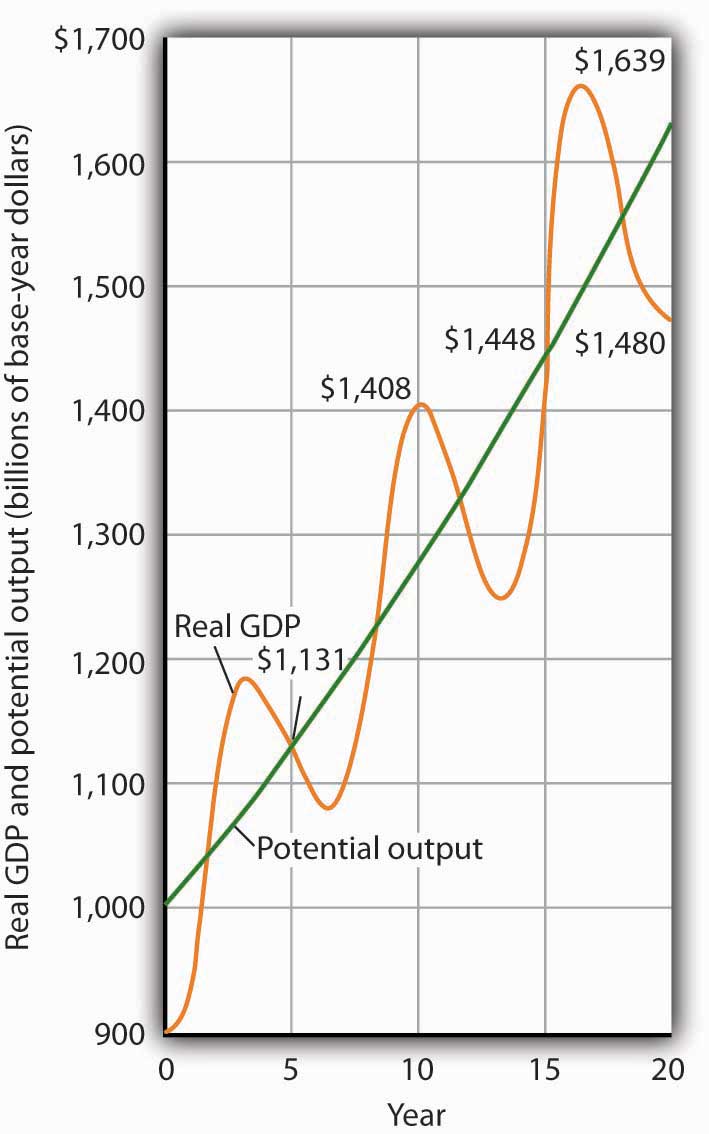
The use of actual values of real GDP to measure growth can give misleading results. Here, an economy’s potential output (shown in green) grows at a steady rate of 2.5% per year, with actual values of real GDP fluctuating about that trend. If we measure growth in the first 10 years as the annual rate of change between beginning and ending values of real GDP, we get a growth rate of 4.6%. The rate for the second decade is 0.5%. Growth estimates based on changes in real GDP are affected by cyclical changes that do not represent economic growth.
Now consider the second decade shown in Figure 8.2 "Cyclical Change Versus Growth". It began in year 10, and it ended in year 20 with a recessionary gap. If we measure the growth rate over that period by looking at beginning and ending values of actual real GDP, we compute an annual growth rate of 0.5%. Viewed in this way, performance in the first decade is spectacular while performance in the second is rather lackluster. But these figures depend on the starting and ending points we select; the growth rate of potential output was 2.5% throughout the period.
By measuring economic growth as the rate of increase in potential output, we avoid such problems. One way to do this is to select years in which the economy was operating at the natural level of employment and then to compute the annual rate of change between those years. The result is an estimate of the rate at which potential output increased over the period in question. For the economy shown in Figure 8.2 "Cyclical Change Versus Growth", for example, we see that real GDP equaled its potential in years 5 and 15. Real GDP in year 5 was $1,131, and real GDP in year 15 was $1,448. The annual rate of change between these two years was 2.5%. If we have estimates of potential output, of course, we can simply compute annual rates of change between any two years.
The Case in Point on presidents and growth at the end of this section suggests a startling fact: the U.S. growth rate began slowing in the 1970s, did not recover until the mid-1990s, only to slow down again in the 2000s. The question we address here is: does it matter? Does a percentage point drop in the growth rate make much difference? It does. To see why, let us investigate what happens when a variable grows at a particular percentage rate.
Suppose two economies with equal populations start out at the same level of real GDP but grow at different rates. Economy A grows at a rate of 3.5%, and Economy B grows at a rate of 2.4%. After a year, the difference in real GDP will hardly be noticeable. After a decade, however, real GDP in Economy A will be 11% greater than in Economy B. Over longer periods, the difference will be more dramatic. After 100 years, for example, income in Economy A will be nearly three times as great as in Economy B. If population growth in the two countries has been the same, the people of Economy A will have a far higher standard of living than those in Economy B. The difference in real GDP per person will be roughly equivalent to the difference that exists today between Great Britain and Mexico.
Over time, small differences in growth rates create large differences in incomes. An economy growing at a 3.5% rate increases by 3.5% of its initial value in the first year. In the second year, the economy increases by 3.5% of that new, higher value. In the third year, it increases by 3.5% of a still higher value. When a quantity grows at a given percentage rate, it experiences exponential growthWhen a quantity grows at a given percentage rate.. A variable that grows exponentially follows a path such as those shown for potential output in Figure 8.1 "A Century of Economic Growth" and Figure 8.2 "Cyclical Change Versus Growth". These curves become steeper over time because the growth rate is applied to an ever-larger base.
A variable growing at some exponential rate doubles over fixed intervals of time. The doubling time is given by the rule of 72A variable’s approximate doubling time equals 72 divided by the growth rate, stated as a whole number., which states that a variable’s approximate doubling time equals 72 divided by the growth rate, stated as a whole number. If the level of income were increasing at a 9% rate, for example, its doubling time would be roughly 72/9, or 8 years.Notice the use of the words roughly and approximately. The actual value of an income of $1,000 growing at rate r for a period of n years is $1,000 × (1 + r)n. After 8 years of growth at a 9% rate, income would thus be $1,000 (1 + 0.09)8 = $1,992.56. The rule of 72 predicts that its value will be $2,000. The rule of 72 gives an approximation, not an exact measure, of the impact of exponential growth.
Let us apply this concept of a doubling time to the reduction in the U.S. growth rate. Had the U.S. economy continued to grow at a 3.5% rate after 1970, then its potential output would have doubled roughly every 20 years (72/3.5 = 20). That means potential output would have doubled by 1990, would double again by 2010, and would double again by 2030. Real GDP in 2030 would thus be eight times as great as its 1970 level. Growing at a 2.4% rate, however, potential output doubles only every 30 years (72/2.4 = 30). It would take until 2000 to double once from its 1970 level, and it would double once more by 2030. Potential output in 2030 would thus be four times its 1970 level if the economy grew at a 2.4% rate (versus eight times its 1970 level if it grew at a 3.5% rate). The 1.1% difference in growth rates produces a 100% difference in potential output by 2030. The different growth paths implied by these growth rates are illustrated in Figure 8.3 "Differences in Growth Rates".
Figure 8.3 Differences in Growth Rates
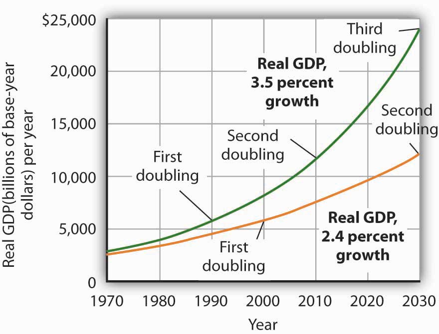
The chart suggests the significance in the long run of a small difference in the growth rate of real GDP. We begin in 1970, when real GDP equaled $2,873.9 billion. If real GDP grew at an annual rate of 3.5% from that year, it would double roughly every 20 years: in 1990, 2010, and 2030. Growth at a 2.4% rate, however, implies doubling every 30 years: in 2000 and 2030. By 2030, the 3.5% growth rate leaves real GDP at twice the level that would be achieved by 2.4% growth.
Of course, it is not just how fast potential output grows that determines how fast the average person’s material standard of living rises. For that purpose, we examine economic growth on a per capita basis. An economy’s output per capitaReal GDP per person. equals real GDP per person. If we let N equal population, then
Equation 8.1
In the United States in the third quarter of 2010, for example, real GDP was $13,277.4 billion (annual rate). The U.S. population was 311.0 million. Real U.S. output per capita thus equaled $42,693.
We use output per capita as a gauge of an economy’s material standard of living. If the economy’s population is growing, then output must rise as rapidly as the population if output per capita is to remain unchanged. If, for example, population increases by 2%, then real GDP would have to rise by 2% to maintain the current level of output per capita. If real GDP rises by less than 2%, output per capita will fall. If real GDP rises by more than 2%, output per capita will rise. More generally, we can write:
Equation 8.2
For economic growth to translate into a higher standard of living on average, economic growth must exceed population growth. From 1970 to 2004, for example, Sierra Leone’s population grew at an annual rate of 2.1% per year, while its real GDP grew at an annual rate of 1.4%; its output per capita thus fell at a rate of 0.7% per year. Over the same period, Singapore’s population grew at an annual rate of 2.1% per year, while its real GDP grew 7.4% per year. The resultant 5.3% annual growth in output per capita transformed Singapore from a relatively poor country to a country with the one of the highest per capita incomes in the world.
Suppose an economy’s potential output and real GDP is $5 million in 2000 and its rate of economic growth is 3% per year. Also suppose that its population is 5,000 in 2000, and that its population grows at a rate of 1% per year. Compute GDP per capita in 2000. Now estimate GDP and GDP per capita in 2072, using the rule of 72. At what rate does GDP per capita grow? What is its doubling time? Is this result consistent with your findings for GDP per capita in 2000 and in 2072?

| President | Annual Increase in Real GDP (%) | Growth Rate (%) |
|---|---|---|
| Truman 1949–1952 | 5.4 | 4.4 |
| Eisenhower 1953–1960 | 2.5 | 3.3 |
| Kennedy-Johnson 1961–1968 | 5.1 | 4.4 |
| Nixon-Ford 1969–1976 | 2.8 | 3.4 |
| Carter 1977–1980 | 3.2 | 3.1 |
| Reagan 1981–1988 | 3.5 | 3.1 |
| G. H. W. Bush 1989–1992 | 2.1 | 2.9 |
| Clinton 1993–2000 | 3.8 | 3.3 |
| G. W. Bush 2001–2008 | 1.6 | 2.6 |
Presidents are often judged by the rate at which the economy grew while they were in office. This test is unfair on two counts. First, a president has little to do with the forces that determine growth. And second, such tests simply compute the annual rate of growth in real GDP over the course of a presidential term, which we know can be affected by cyclical factors. A president who takes office when the economy is down and goes out with the economy up will look like an economic star; a president with the bad luck to have reverse circumstances will seem like a dud. Here are annual rates of change in real GDP for each of the postwar presidents, together with rates of economic growth, measured as the annual rate of change in potential output.
The presidents’ economic records are clearly affected by luck. Presidents Truman, Kennedy, Reagan, and Clinton, for example, began their terms when the economy had a recessionary gap and ended them with an inflationary gap or at about potential output. Real GDP thus rose faster than potential output during their presidencies. The Eisenhower, Nixon-Ford, G. H. W. Bush, and G. W. Bush administrations each started with an inflationary gap or at about potential and ended with a recessionary gap, thus recording rates of real GDP increase below the rate of gain in potential. Only Jimmy Carter, who came to office and left it with recessionary gaps, presided over a relatively equivalent rate of increase in actual GDP versus potential output.
How did Barack Obama fare? As this case was written after he was in office for less than a full term, you will have to check for yourself!
GDP per capita in 2000 equals $1,000 ($5,000,000/5,000). If GDP rises 3% per year, it doubles every 24 years (= 72/3). Thus, GDP will be $10,000,000 in 2024, $20,000,000 in 2048, and $40,000,000 in 2072. Growing at a rate of 1% per year, population will have doubled once by 2072 to 10,000. GDP per capita will thus be $4,000 (= $40,000,000/10,000). Notice that GDP rises by eight times its original level, while the increase in GDP per capita is fourfold. The latter value represents a growth rate in output per capita of 2% per year, which implies a doubling time of 36 years. That gives two doublings in GDP per capita between 2000 and 2072 and confirms a fourfold increase.
Economic growth means the economy’s potential output is rising. Because the long-run aggregate supply curve is a vertical line at the economy’s potential, we can depict the process of economic growth as one in which the long-run aggregate supply curve shifts to the right.
Figure 8.4 Economic Growth and the Long-Run Aggregate Supply Curve

Because economic growth is the process through which the economy’s potential output is increased, we can depict it as a series of rightward shifts in the long-run aggregate supply curve. Notice that with exponential growth, each successive shift in LRAS is larger and larger.
Figure 8.4 "Economic Growth and the Long-Run Aggregate Supply Curve" illustrates the process of economic growth. If the economy begins at potential output of Y1, growth increases this potential. The figure shows a succession of increases in potential to Y2, then Y3, and Y4. If the economy is growing at a particular percentage rate, and if the levels shown represent successive years, then the size of the increases will become larger and larger, as indicated in the figure.
Because economic growth can be considered as a process in which the long-run aggregate supply curve shifts to the right, and because output tends to remain close to this curve, it is important to gain a deeper understanding of what determines long-run aggregate supply (LRAS). We shall examine the derivation of LRAS and then see what factors shift the curve. We shall begin our work by defining an aggregate production function.
An aggregate production functionFunction that relates the total output of an economy to the total amount of labor employed in the economy, all other determinants of production (capital, natural resources, and technology) being unchanged. relates the total output of an economy to the total amount of labor employed in the economy, all other determinants of production (that is, capital, natural resources, and technology) being unchanged. An economy operating on its aggregate production function is producing its potential level of output.
Figure 8.5 "The Aggregate Production Function" shows an aggregate production function (PF). It shows output levels for a range of employment between 120 million and 140 million workers. When the level of employment is 120 million, the economy produces a real GDP of $11,500 billion (point A). A level of employment of 130 million produces a real GDP of $12,000 billion (point B), and when 140 million workers are employed, a real GDP of $12,300 billion is produced (point C). In drawing the aggregate production function, the amount of labor varies, but everything else that could affect output, specifically the quantities of other factors of production and technology, is fixed.
The shape of the aggregate production function shows that as employment increases, output increases, but at a decreasing rate. Increasing employment from 120 million to 130 million, for example, increases output by $500 billion to $12,000 billion at point B. The next 10 million workers increase production by $300 billion to $12,300 billion at point C. This example illustrates diminishing marginal returns. Diminishing marginal returnsSituation that occurs when additional units of a variable factor add less and less to total output, given constant quantities of other factors. occur when additional units of a variable factor add less and less to total output, given constant quantities of other factors.
Figure 8.5 The Aggregate Production Function
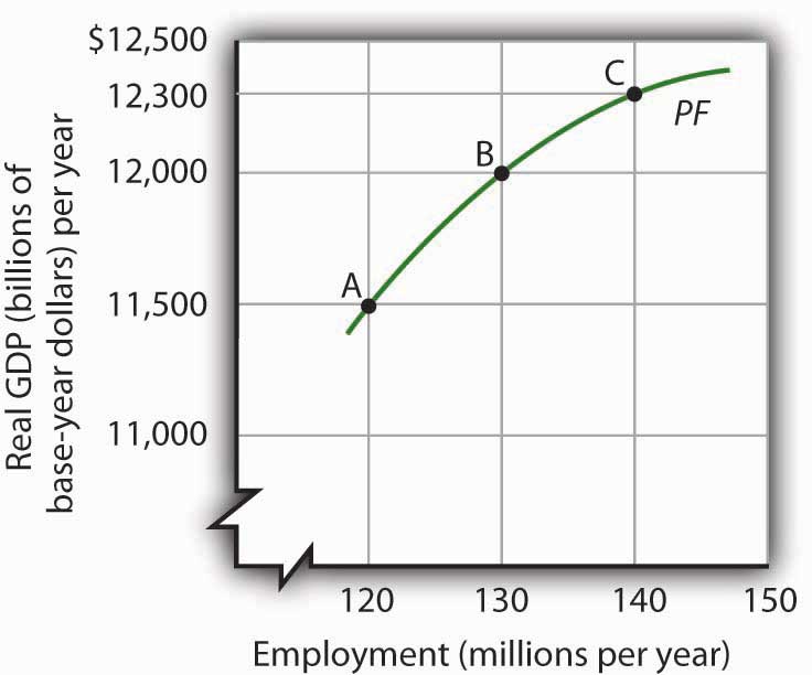
An aggregate production function (PF) relates total output to total employment, assuming all other factors of production and technology are fixed. It shows that increases in employment lead to increases in output but at a decreasing rate.
It is easy to picture the problem of diminishing marginal returns in the context of a single firm. The firm is able to increase output by adding workers. But because the firm’s plant size and stock of equipment are fixed, the firm’s capital per worker falls as it takes on more workers. Each additional worker adds less to output than the worker before. The firm, like the economy, experiences diminishing marginal returns.
To derive the long-run aggregate supply curve, we bring together the model of the labor market, introduced in the first macro chapter and the aggregate production function.
As we learned, the labor market is in equilibrium at the natural level of employment. The demand and supply curves for labor intersect at the real wage at which the economy achieves its natural level of employment. We see in Panel (a) of Figure 8.6 "Deriving the Long-Run Aggregate Supply Curve" that the equilibrium real wage is ω1 and the natural level of employment is L1. Panel (b) shows that with employment of L1, the economy can produce a real GDP of YP. That output equals the economy’s potential output. It is that level of potential output that determines the position of the long-run aggregate supply curve in Panel (c).
Figure 8.6 Deriving the Long-Run Aggregate Supply Curve
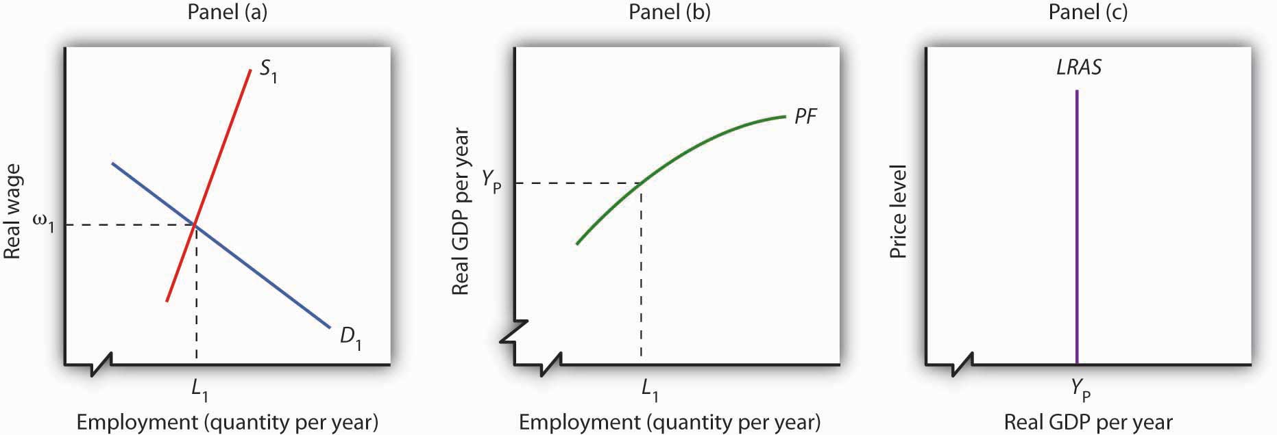
Panel (a) shows that the equilibrium real wage is ω1, and the natural level of employment is L1. Panel (b) shows that with employment of L1, the economy can produce a real GDP of YP. That output equals the economy’s potential output. It is at that level of potential output that we draw the long-run aggregate supply curve in Panel (c).
The position of the long-run aggregate supply curve is determined by the aggregate production function and the demand and supply curves for labor. A change in any of these will shift the long-run aggregate supply curve.
Figure 8.7 "Shift in the Aggregate Production Function and the Long-Run Aggregate Supply Curve" shows one possible shifter of long-run aggregate supply: a change in the production function. Suppose, for example, that an improvement in technology shifts the aggregate production function in Panel (b) from PF1 to PF2. Other developments that could produce an upward shift in the curve include an increase in the capital stock or in the availability of natural resources.
Figure 8.7 Shift in the Aggregate Production Function and the Long-Run Aggregate Supply Curve
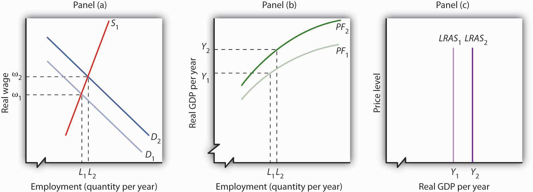
An improvement in technology shifts the aggregate production function upward in Panel (b). Because labor is more productive, the demand for labor shifts to the right in Panel (a), and the natural level of employment increases to L2. In Panel (c) the long-run aggregate supply curve shifts to the right to Y2.
The shift in the production function to PF2 means that labor is now more productive than before. This will affect the demand for labor in Panel (a). Before the technological change, firms employed L1 workers at a real wage ω1. If workers are more productive, firms will find it profitable to hire more of them at ω1. The demand curve for labor thus shifts to D2 in Panel (a). The real wage rises to ω2, and the natural level of employment rises to L2. The increase in the real wage reflects labor’s enhanced productivityThe amount of output per worker., the amount of output per worker. To see how potential output changes, we see in Panel (b) how much output can be produced given the new natural level of employment and the new aggregate production function. The real GDP that the economy is capable of producing rises from Y1 to Y2. The higher output is a reflection of a higher natural level of employment, along with the fact that labor has become more productive as a result of the technological advance. In Panel (c) the long-run aggregate supply curve shifts to the right to the vertical line at Y2.
This analysis dispels a common misconception about the impact of improvements in technology or increases in the capital stock on employment. Some people believe that technological gains or increases in the stock of capital reduce the demand for labor, reduce employment, and reduce real wages. Certainly the experience of the United States and most other countries belies that notion. Between 1990 and 2007, for example, the U.S. capital stock and the level of technology increased dramatically. During the same period, employment and real wages rose, suggesting that the demand for labor increased by more than the supply of labor. As some firms add capital or incorporate new technologies, some workers at those firms may lose their jobs. But for the economy as a whole, new jobs become available and they generally offer higher wages. The demand for labor rises.
Another event that can shift the long-run aggregate supply curve is an increase in the supply of labor, as shown in Figure 8.8 "Increase in the Supply of Labor and the Long-Run Aggregate Supply Curve". An increased supply of labor could result from immigration, an increase in the population, or increased participation in the labor force by the adult population. Increased participation by women in the labor force, for example, has tended to increase the supply curve for labor during the past several decades.
Figure 8.8 Increase in the Supply of Labor and the Long-Run Aggregate Supply Curve
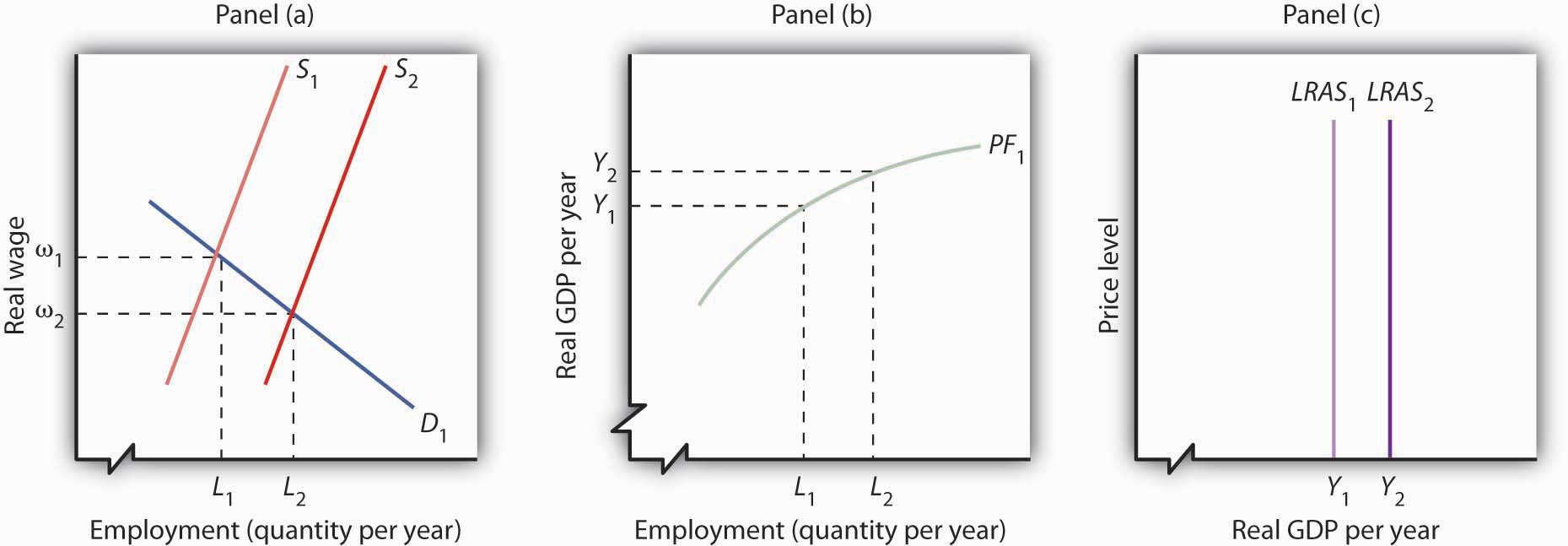
An increase in the supply of labor shifts the supply curve in Panel (a) to S2, and the natural level of employment rises to L2. The real wage falls to ω2. With increased labor, the aggregate production function in Panel (b) shows that the economy is now capable of producing real GDP at Y2. The long-run aggregate supply curve in Panel (c) shifts to LRAS2.
In Panel (a), an increase in the labor supply shifts the supply curve to S2. The increase in the supply of labor does not change the stock of capital or natural resources, nor does it change technology—it therefore does not shift the aggregate production function. Because there is no change in the production function, there is no shift in the demand for labor. The real wage falls from ω1 to ω2 in Panel (a), and the natural level of employment rises from L1 to L2. To see the impact on potential output, Panel (b) shows that employment of L2 can produce real GDP of Y2. The long-run aggregate supply curve in Panel (c) thus shifts to LRAS2. Notice, however, that this shift in the long-run aggregate supply curve to the right is associated with a reduction in the real wage to ω2.
Of course, the aggregate production function and the supply curve of labor can shift together, producing higher real wages at the same time population rises. That has been the experience of most industrialized nations. The increase in real wages in the United States between 1990 and 2007, for example, came during a period in which an increasing population increased the supply of labor. The demand for labor increased by more than the supply, pushing the real wage up. The accompanying Case in Point looks at gains in real wages in the face of technological change, an increase in the stock of capital, and rapid population growth in the United States during the 19th century.
Our model of long-run aggregate supply tells us that in the long run, real GDP, the natural level of employment, and the real wage are determined by the economy’s production function and by the demand and supply curves for labor. Unless an event shifts the aggregate production function, the demand curve for labor, or the supply curve for labor, it affects neither the natural level of employment nor potential output. Economic growth occurs only if an event shifts the economy’s production function or if there is an increase in the demand for or the supply of labor.
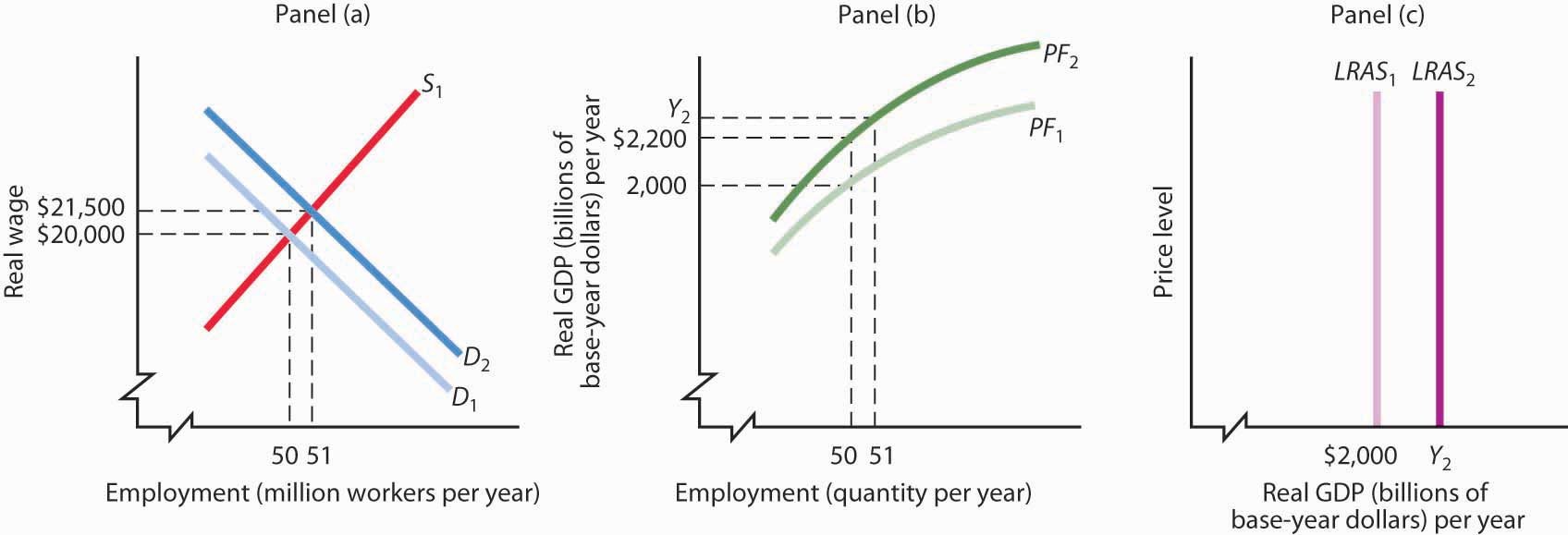
Suppose that the quantity of labor supplied is 50 million workers when the real wage is $20,000 per year and that potential output is $2,000 billion per year. Draw a three-panel graph similar to the one presented in Figure 8.8 "Increase in the Supply of Labor and the Long-Run Aggregate Supply Curve" to show the economy’s long-run equilibrium. Panel (a) of your graph should show the demand and supply curves for labor, Panel (b) should show the aggregate production function, and Panel (c) should show the long-run aggregate supply curve. Now suppose a technological change increases the economy’s output with the same quantity of labor as before to $2,200 billion, and the real wage rises to $21,500. In response, the quantity of labor supplied increases to 51 million workers. In the same three panels you have already drawn, sketch the new curves that result from this change. Explain what happens to the level of employment, the level of potential output, and the long-run aggregate supply curve. (Hint: you have information for only one point on each of the curves you draw—two for the supply of labor; simply draw curves of the appropriate shape. Do not worry about getting the scale correct.)
Technological change and the capital investment that typically comes with it are often criticized because they replace labor with machines, reducing employment. Such changes, critics argue, hurt workers. Using the model of aggregate demand and aggregate supply, however, we arrive at a quite different conclusion. The model predicts that improved technology will increase the demand for labor and boost real wages.
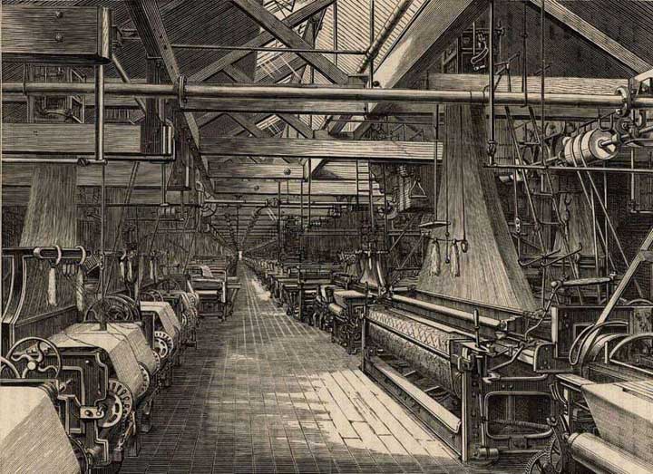
The period of industrialization, generally taken to be the time between the Civil War and World War I, was a good test of these competing ideas. Technological changes were dramatic as firms shifted toward mass production and automation. Capital investment soared. Immigration increased the supply of labor. What happened to workers?
Employment more than doubled during this period, consistent with the prediction of our model. It is harder to predict, from a theoretical point of view, the consequences for real wages. The latter third of the 19th century was a period of massive immigration to the United States. Between 1865 and 1880, more than 5 million people came to the United States from abroad; most were of working age. The pace accelerated between 1880 and 1923, when more than 23 million people moved to the United States from other countries. Immigration increased the supply of labor, which should reduce the real wage. There were thus two competing forces at work: Technological change and capital investment tended to increase real wages, while immigration tended to reduce them by increasing the supply of labor.
The evidence suggests that the forces of technological change and capital investment proved far more powerful than increases in labor supply. Real wages soared 60% between 1860 and 1890. They continued to increase after that. Real wages in manufacturing, for example, rose 37% from 1890 to 1914.
Technological change and capital investment displace workers in some industries. But for the economy as a whole, they increase worker productivity, increase the demand for labor, and increase real wages.
Sources: Wage data taken from Clarence D. Long, Wages and Earnings in the United States, 1860–1990 (Princeton, NJ: Princeton University Press, 1960), p. 109, and from Albert Rees, Wages in Manufacturing, 1890–1914 (Princeton, NJ: Princeton University Press, 1961), pp. 3–5. Immigration figures taken from Gary M. Walton and Hugh Rockoff, History of the American Economy, 6th ed. (New York: Harcourt Brace Jovanovich, 1990), p. 371.
The production function in Panel (b) shifts up to PF2. Because it reflects greater productivity of labor, firms will increase their demand for labor, and the demand curve for labor shifts to D2 in Panel (a). LRAS1 shifts to LRAS2 in Panel (c). Employment and potential output rise. Potential output will be greater than $2,200 billion.
In this section, we review the main determinants of economic growth. We also examine the reasons for the widening disparities in economic growth rates among countries in recent years.
As we have learned, there are two ways to model economic growth: (1) as an outward shift in an economy’s production possibilities curve, and (2) as a shift to the right in its long-run aggregate supply curve. In drawing either one at a point in time, we assume that the economy’s factors of production and its technology are unchanged. Changing these will shift both curves. Therefore, anything that increases the quantity or quality of factors of production or that improves the technology available to the economy contributes to economic growth.
The sources of growth for the U.S. economy in the 20th century were presented in the chapter on choices in production. There we learned that the main sources of growth for the United States from 1960 to 2007 were divided between increases in the quantities of labor and of physical capital (about 65%) and in improvements in the qualities of the factors of production and technology (about 35%). Since 2000, however, the contributions from improvements in factor quality and technology have accounted for about half the economic growth in the United States.
In order to devote resources to increasing physical and human capital and to improving technology—activities that will enhance future production—society must forgo using them now to produce consumer goods. Even though the people in the economy would enjoy a higher standard of living today without this sacrifice, they are willing to reduce present consumption in order to have more goods and services available for the future.
As a college student, you personally made such a choice. You decided to devote time to study that you could have spent earning income. With the higher income, you could enjoy greater consumption today. You made this choice because you expect to earn higher income in the future and thus to enjoy greater consumption in the future. Because many other people in the society also choose to acquire more education, society allocates resources to produce education. The education produced today will enhance the society’s human capital and thus its economic growth.
All other things equal, higher saving allows more resources to be devoted to increases in physical and human capital and technological improvement. In other words, saving, which is income not spent on consumption, promotes economic growth by making available resources that can be channeled into growth-enhancing uses.
Toward the end of the 20th century, it appeared that some of the world’s more affluent countries were growing robustly while others were growing more slowly or even stagnating. This observation was confirmed in a major study by the Organisation for Economic Co-operation and Development (OECD),The material in this section is based on Organisation for Economic Co-operation and Development, The Sources of Economic Growth in OECD Countries, 2003. whose members are listed in Table 8.1 "Growing Disparities in Rates of Economic Growth". The table shows that for the OECD countries as a whole, economic growth per capita fell from an average of 2.2% per year in the 1980s to an average of 1.9% per year in the 1990s. The higher standard deviation in the latter period confirms an increased disparity of growth rates in the more recent period. Moreover, the data on individual countries show that per capita growth in some countries (specifically, the United States, Canada, Ireland, Netherlands, Norway, and Spain) picked up, especially in the latter half of the 1990s, while it decelerated in most of the countries of continental Europe and Japan.
Table 8.1 Growing Disparities in Rates of Economic Growth
| Trend Growth of GDP per Capita | |||
|---|---|---|---|
| Country | 1980–1990 | 1990–2000 | 1996–2000 |
| United States | 2.1 | 2.3 | 2.8 |
| Japan | 3.3 | 1.4 | 0.9 |
| Germany | 1.9 | 1.2 | 1.7 |
| France | 1.6 | 1.5 | 1.9 |
| Italy | 2.3 | 1.5 | 1.7 |
| United Kingdom | 2.2 | 2.1 | 2.3 |
| Canada | 1.4 | 1.7 | 2.6 |
| Austria | 2.1 | 1.9 | 2.3 |
| Belgium | 2.0 | 1.9 | 2.3 |
| Denmark | 1.9 | 1.9 | 2.3 |
| Finland | 2.2 | 2.1 | 3.9 |
| Greece | 0.5 | 1.8 | 2.7 |
| Iceland | 1.7 | 1.5 | 2.6 |
| Ireland | 3.0 | 6.4 | 7.9 |
| Luxembourg | 4.0 | 4.5 | 4.6 |
| Netherlands | 1.6 | 2.4 | 2.7 |
| Portugal | 3.1 | 2.8 | 2.7 |
| Spain | 2.3 | 2.7 | 3.2 |
| Sweden | 1.7 | 1.5 | 2.6 |
| Switzerland | 1.4 | 0.4 | 1.1 |
| Turkey | 2.1 | 2.1 | 1.9 |
| Australia | 1.6 | 2.4 | 2.8 |
| New Zealand | 1.4 | 1.2 | 1.8 |
| Mexico | 0.0 | 1.6 | 2.7 |
| Korea | 7.2 | 5.1 | 4.2 |
| Hungary | — | 2.3 | 3.5 |
| Poland | — | 4.2 | 4.8 |
| Czech Republic | — | 1.7 | 1.4 |
| OECD24* | 2.2 | 1.9 | 2.2 |
| Standard Deviation of OECD24 | 0.74 | 1.17 | 1.37 |
| *Excludes Czech Republic, Hungary, Korea, Mexico, Poland, and Slovak Republic | |||
Variation in the growth in real GDP per capita has widened among the world’s leading industrialized economies.
Source: Excerpted from Table 1.1 Organisation for Economic Co-operation and Development, Sources of Economic Growth in OECD Countries, 2003: p. 32–33.
The study goes on to try to explain the reasons for the divergent growth trends. The main findings were:
The general concern in the second half of the 1970s and the 1980s was that economic growth was slowing down and that it might not be possible to reverse this pattern. The 1990s and early 2000s, in which growth picked up in some countries but not in others, suggested that the problem was not universal and led to a search for the reasons for the disparities in growth rates that emerged. The OECD study described above gives some possible explanations. The findings of that study practically beg countries to examine closely their economic policies at a variety of levels and to consider changes that may add flexibility to their economies.
To spur this process, in 2005, the OECD started a new annual publication called Going for Growth. The inaugural edition identified five priority structural policy areas specific to each OECD country. The policies were categorized as either improving labor utilization or improving productivity. Suggestions for improved labor utilization ranged from changing tax policies to improving incentives for females to enter, and for older people to remain in, the workforce. Suggestions for improved productivity ranged from education reform to privatization of state-owned industries. As an example, the priorities proposed for the United States in 2005 included (1) limiting increases in labor costs by reforming Medicare to restrain health care costs, (2) encouraging private saving by shifting the burden of taxation toward consumption, (3) improving primary and secondary education, (4) reducing trade-distorting agricultural price supports, and (5) promoting transparency and accountability of corporate governance.Organisation for Economic Co-operation and Development, Economic Policy Reforms: Going for Growth 2005, available at http://www.OECD.org/economics/goingforgrowth.
The 2010 edition of Going for GrowthOrganisation for Economic Co-operation and Development, Economic Policy Reforms: Going for Growth 2010, available at http://www.OECD.org/economics/goingforgrowth. took stock of the progress made over the five-year period leading up to 2010. While two-thirds of the OECD countries took some legislative action in at least one priority area, the scope and depth of this progress varied immensely across countries.
Figure 8.9 " of " summarizes this progress using two alternative measures. Panel (a) shows a responsiveness rate, which measures significant actions taken, and Panel (b) shows a follow-through rate, which measures whether priorities could be dropped due to reform implementation.
As we can see, the responsiveness and follow-through rates vary widely. Turkey and the Czech Republic stand out as the countries having undertaken substantial reform. The United States stands out as the country having shown neither responsiveness nor follow-through. While the relatively strong performance of the United States at the end of the 20th century, as shown in Table 8.1 "Growing Disparities in Rates of Economic Growth", could indicate relatively less need for growth-enhancing reforms, the comparative lack of progress since 2005 raises doubt concerning the ability to maintain strong economic growth going forward.
Figure 8.9 of Going for Growth Recommendations across Countries since 2005
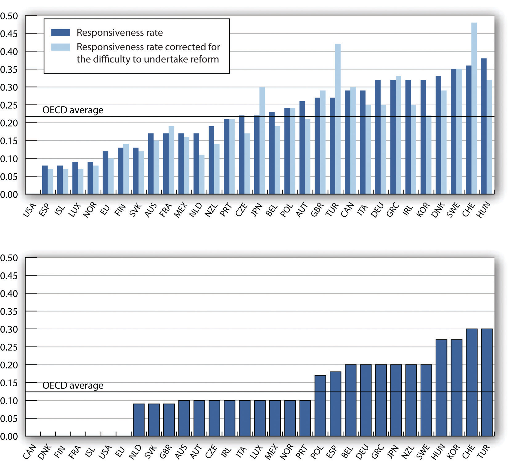
Panel (a) measures the 2005 to 2009 rate of responsiveness to the reform priorities given to each country in 2005. Panel (b) shows the reform follow-through rates. Growth-enhancing policy reforms across countries varied widely during this period.
Source: Organisation for Economic Co-operation and Development, Going for Growth 2010, Figure 2.6, p. 75.
In closing, it is worth reiterating that economic freedom and higher incomes tend to go together. Countries could not have attained high levels of income if they had not maintained the economic freedom that contributed to high incomes in the first place. Thus, it is also likely that rates of economic growth in the future will be related to the amount of economic freedom countries choose. We shall see in later chapters that monetary and fiscal policies that are used to stabilize the economy in the short run can also have an impact on long-run economic growth.
All other things unchanged, compare the position of a country’s expected production possibility curve and the expected position of its long-run aggregate supply curve if:

Economist William Easterly in his aptly named book The Elusive Quest for Growth: Economists’ Adventures and Misadventures in the Tropics admits that after 50 years of searching for the magic formula for turning poor countries into rich ones, the quest remains elusive.
Poor countries just need more physical capital, you say? Easterly points out that between 1960 and 1985, the capital stock per worker in both Gambia and Japan rose by over 500%. The result? In Gambia, output per worker over the 25-year period rose 2%; in Japan, output per worker rose 260%.
So, it must be that poor countries need more human capital? Again, he finds startling comparisons. For example, human capital expanded faster in Zambia than in Korea, but Zambia’s annual growth rate is 7 percentage points below Korea’s.
Too much population growth? Too little? More foreign aid? Too much? As Easterly proceeds, writing a prescription for growth seems ever more difficult: “None has delivered as promised,” he concludes (p. xi).
While Easterly does not offer his own new panacea for how to move countries to a higher level of per capita GDP, where the model presented in this chapter does seem to provide some explanations of why a country’s growth rate may vary over time or differ from another country’s, he does argue that creating incentives for growth in poor countries is crucial. Acknowledging a role for plain luck, Easterly argues that good government policies—ones that keep low such negatives as inflation, corruption, and red tape—and quality institutions and laws—ones that, for example, honor contracts and reward merit—will help.
How to actually improve such incentives might constitute the next great quest:
“We have learned once and for all that there are no magical elixirs to bring a happy ending to our quest for growth. Prosperity happens when all the players in the development game have the right incentives. It happens when government incentives induce technological adaptation, high-quality investment in machines, and high-quality schooling. It happens when donors face incentives that induce them to give aid to countries with good policies where aid will have high payoffs, not to countries with poor policies where aid is wasted. It happens when the poor get good opportunities and incentives, which requires government welfare programs that reward rather than penalize earning income. It happens when politics is not polarized between antagonistic interest groups. . . . The solutions are a lot more difficult to describe than the problems. The way forward must be to create incentives for growth for the trinity of governments, donors, and individuals.” (p. 289–90)
Source: William Easterly, The Elusive Quest for Growth: Economists’ Adventures and Misadventures in the Tropics (Cambridge: MIT Press, 2002).
Situations 1 and 4 should lead to a shift further outward in the country’s production possibility curve and further to the right in its long-run aggregate supply curve. Situations 2 and 3 should lead to smaller outward shifts in the country’s production possibility curve and smaller rightward shifts in its long-run aggregate supply curve.
We saw that economic growth can be measured by the rate of increase in potential output. Measuring the rate of increase in actual real GDP can confuse growth statistics by introducing elements of cyclical variation.
Growth is an exponential process. A variable increasing at a fixed percentage rate doubles over fixed intervals. The doubling time is approximated by the rule of 72. The exponential nature of growth means that small differences in growth rates have large effects over long periods of time. Per capita rates of increase in real GDP are found by subtracting the growth rate of the population from the growth rate of GDP.
Growth can be shown in the model of aggregate demand and aggregate supply as a series of rightward shifts in the long-run aggregate supply curve. The position of the LRAS is determined by the aggregate production function and by the demand and supply curves for labor. A rightward shift in LRAS results either from an upward shift in the production function, due to increases in factors of production other than labor or to improvements in technology, or from an increase in the demand for or the supply of labor.
Saving plays an important role in economic growth, because it allows for more capital to be available for future production, so the rate of economic growth can rise. Saving thus promotes growth.
In recent years, rates of growth among the world’s industrialized countries have grown more disparate. Recent research suggests this may be related to differing labor and product market conditions, differences in the diffusion of information and communications technologies, as well as differences in macroeconomic and trade policies. Evidence on the role that government plays in economic growth was less conclusive.
The population of the world in 2003 was 6.314 billion. It grew between 1975 and 2003 at an annual rate of 1.6%. Assume that it continues to grow at this rate.
With a world population in 2003 of 6.314 billion and a projected population growth rate of 1.1% instead (which is the United Nations’ projection for the period 2003 to 2015).
Suppose a country’s population grows at the rate of 2% per year and its output grows at the rate of 3% per year.
The rate of economic growth per capita in France from 1996 to 2000 was 1.9% per year, while in Korea over the same period it was 4.2%. Per capita real GDP was $28,900 in France in 2003, and $12,700 in Korea. Assume the growth rates for each country remain the same.
Suppose real GDPs in country A and country B are identical at $10 trillion dollars in 2005. Suppose country A’s economic growth rate is 2% and country B’s is 4% and both growth rates remain constant over time.
Suppose country A’s population grows 1% per year and country B’s population grows 3% per year.
Suppose the information below characterizes an economy:
| Employment (in millions) | Real GDP (in billions) |
|---|---|
| 1 | 200 |
| 2 | 700 |
| 3 | 1,100 |
| 4 | 1,400 |
| 5 | 1,650 |
| 6 | 1,850 |
| 7 | 2,000 |
| 8 | 2,100 |
| 9 | 2,170 |
| 10 | 2,200 |
Suppose that improvement in technology means that real GDP at each level of employment rises by $200 billion.
In Table 8.1 "Growing Disparities in Rates of Economic Growth", we can see that Japan’s growth rate of per capita real GDP fell from 3.3% per year in the 1980s to 1.4% per year in the 1990s.


