For nearly three decades, Americans have come to expect very low inflation, on the order of 2% to 3% a year. How did this expectation come to be? Was it always so? Absolutely not.
In July 1979, with inflation approaching 14% and interest rates on three-month Treasury bills soaring past 10%, a desperate President Jimmy Carter took action. He appointed Paul Volcker, the president of the New York Federal Reserve Bank, as chairman of the Fed’s Board of Governors. Mr. Volcker made clear that his objective as chairman was to bring down the inflation rate—no matter what the consequences for the economy. Mr. Carter gave this effort his full support.
Mr. Volcker wasted no time in putting his policies to work. He slowed the rate of money growth immediately. The economy’s response was swift; the United States slipped into a brief recession in 1980, followed by a crushing recession in 1981–1982. In terms of the goal of reducing inflation, Mr. Volcker’s monetary policies were a dazzling success. Inflation plunged below a 4% rate within three years; by 1986 the inflation rate had fallen to 1.1%. The tall, bald, cigar-smoking Mr. Volcker emerged as a folk hero in the fight against inflation. Indeed he has returned 20 years later as part of President Obama’s economic team to perhaps once again rescue the U.S. economy.
The Fed’s seven-year fight against inflation from 1979 to 1986 made the job for Alan Greenspan, Mr. Volcker’s successor, that much easier. To see how the decisions of the Federal Reserve affect key macroeconomic variables—real GDP, the price level, and unemployment—in this chapter we will explore how financial marketsMarkets in which funds accumulated by one group are made available to another group., markets in which funds accumulated by one group are made available to another group, are linked to the economy.
This chapter provides the building blocks for understanding financial markets. Beginning with an overview of bond and foreign exchange markets, we will examine how they are related to the level of real GDP and the price level. The second section completes the model of the money market. We have learned that the Fed can change the amount of reserves in the banking system, and that when it does the money supply changes. Here we explain money demand—the quantity of money people and firms want to hold—which, together with money supply, leads to an equilibrium rate of interest.
The model of aggregate demand and supply shows how changes in the components of aggregate demand affect GDP and the price level. In this chapter, we will learn that changes in the financial markets can affect aggregate demand—and in turn can lead to changes in real GDP and the price level. Showing how the financial markets fit into the model of aggregate demand and aggregate supply we developed earlier provides a more complete picture of how the macroeconomy works.
In this section, we will look at the bond market and at the market for foreign exchange. Events in these markets can affect the price level and output for the entire economy.
In their daily operations and in pursuit of new projects, institutions such as firms and governments often borrow. They may seek funds from a bank. Many institutions, however, obtain credit by selling bonds. The federal government is one institution that issues bonds. A local school district might sell bonds to finance the construction of a new school. Your college or university has probably sold bonds to finance new buildings on campus. Firms often sell bonds to finance expansion. The market for bonds is an enormously important one.
When an institution sells a bond, it obtains the price paid for the bond as a kind of loan. The institution that issues the bond is obligated to make payments on the bond in the future. The interest rate is determined by the price of the bond. To understand these relationships, let us look more closely at bond prices and interest rates.
Suppose the manager of a manufacturing company needs to borrow some money to expand the factory. The manager could do so in the following way: he or she prints, say, 500 pieces of paper, each bearing the company’s promise to pay the bearer $1,000 in a year. These pieces of paper are bonds, and the company, as the issuer, promises to make a single payment. The manager then offers these bonds for sale, announcing that they will be sold to the buyers who offer the highest prices. Suppose the highest price offered is $950, and all the bonds are sold at that price. Each bond is, in effect, an obligation to repay buyers $1,000. The buyers of the bonds are being paid $50 for the service of lending $950 for a year.
The $1,000 printed on each bond is the face value of the bondThe amount the issuer of a bond will have to pay on the maturity date.; it is the amount the issuer will have to pay on the maturity dateThe date when a bond matures, or comes due. of the bond—the date when the loan matures, or comes due. The $950 at which they were sold is their price. The difference between the face value and the price is the amount paid for the use of the money obtained from selling the bond.
An interest ratePayment made for the use of money, expressed as a percentage of the amount borrowed. is the payment made for the use of money, expressed as a percentage of the amount borrowed. Bonds you sold command an interest rate equal to the difference between the face value and the bond price, divided by the bond price, and then multiplied by 100 to form a percentage:
Equation 10.1
At a price of $950, the interest rate is 5.3%
The interest rate on any bond is determined by its price. As the price falls, the interest rate rises. Suppose, for example, that the best price the manager can get for the bonds is $900. Now the interest rate is 11.1%. A price of $800 would mean an interest rate of 25%; $750 would mean an interest rate of 33.3%; a price of $500 translates into an interest rate of 100%. The lower the price of a bond relative to its face value, the higher the interest rate.
Bonds in the real world are more complicated than the piece of paper in our example, but their structure is basically the same. They have a face value (usually an amount between $1,000 and $100,000) and a maturity date. The maturity date might be three months from the date of issue; it might be 30 years.
Whatever the period until it matures, and whatever the face value of the bond may be, its issuer will attempt to sell the bond at the highest possible price. Buyers of bonds will seek the lowest prices they can obtain. Newly issued bonds are generally sold in auctions. Potential buyers bid for the bonds, which are sold to the highest bidders. The lower the price of the bond relative to its face value, the higher the interest rate.
Both private firms and government entities issue bonds as a way of raising funds. The original buyer need not hold the bond until maturity. Bonds can be resold at any time, but the price the bond will fetch at the time of resale will vary depending on conditions in the economy and the financial markets.
Figure 10.1 "The Bond Market" illustrates the market for bonds. Their price is determined by demand and supply. Buyers of newly issued bonds are, in effect, lenders. Sellers of newly issued bonds are borrowers—recall that corporations, the federal government, and other institutions sell bonds when they want to borrow money. Once a newly issued bond has been sold, its owner can resell it; a bond may change hands several times before it matures.
Figure 10.1 The Bond Market
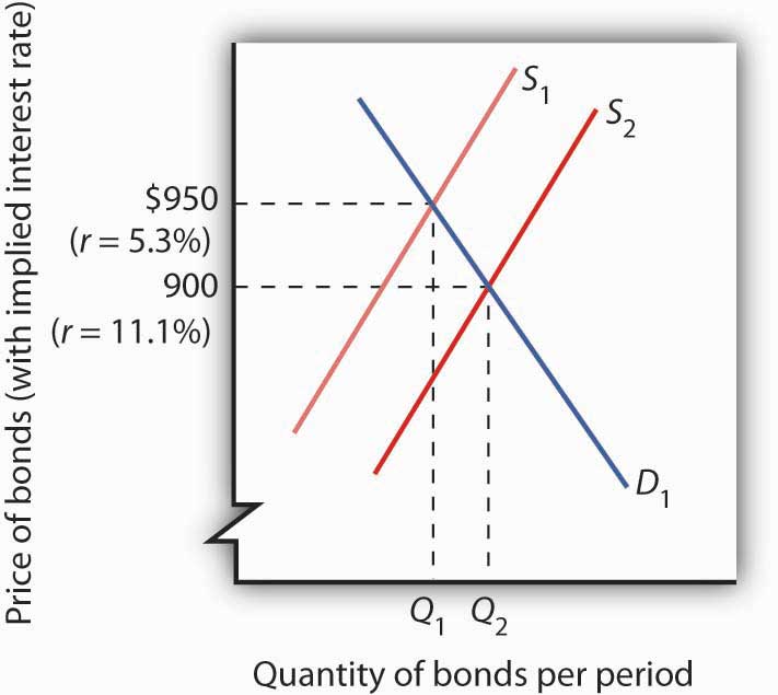
The equilibrium price for bonds is determined where the demand and supply curves intersect. The initial solution here is a price of $950, implying an interest rate of 5.3%. An increase in borrowing, all other things equal, increases the supply of bonds to S2 and forces the price of bonds down to $900. The interest rate rises to 11.1%.
Bonds are not exactly the same sort of product as, say, broccoli or some other good or service. Can we expect bonds to have the same kind of downward-sloping demand curves and upward-sloping supply curves we encounter for ordinary goods and services? Yes. Consider demand. At lower prices, bonds pay higher interest. That makes them more attractive to buyers of bonds and thus increases the quantity demanded. On the other hand, lower prices mean higher costs to borrowers—suppliers of bonds—and should reduce the quantity supplied. Thus, the negative relationship between price and quantity demanded and the positive relationship between price and quantity supplied suggested by conventional demand and supply curves holds true in the market for bonds.
If the quantity of bonds demanded is not equal to the quantity of bonds supplied, the price will adjust almost instantaneously to balance the two. Bond prices are perfectly flexible in that they change immediately to balance demand and supply. Suppose, for example, that the initial price of bonds is $950, as shown by the intersection of the demand and supply curves in Figure 10.1 "The Bond Market". We will assume that all bonds have equal risk and a face value of $1,000 and that they mature in one year. Now suppose that borrowers increase their borrowing by offering to sell more bonds at every interest rate. This increases the supply of bonds: the supply curve shifts to the right from S1 to S2. That, in turn, lowers the equilibrium price of bonds—to $900 in Figure 10.1 "The Bond Market". The lower price for bonds means a higher interest rate.
The connection between the bond market and the economy derives from the way interest rates affect aggregate demand. For example, investment is one component of aggregate demand, and interest rates affect investment. Firms are less likely to acquire new capital (that is, plant and equipment) if interest rates are high; they’re more likely to add capital if interest rates are low.Consumption may also be affected by changes in interest rates. For example, if interest rates fall, consumers can more easily obtain credit and thus are more likely to purchase cars and other durable goods. To simplify, we ignore this effect.
If bond prices fall, interest rates go up. Higher interest rates tend to discourage investment, so aggregate demand will fall. A fall in aggregate demand, other things unchanged, will mean fewer jobs and less total output than would have been the case with lower rates of interest. In contrast, an increase in the price of bonds lowers interest rates and makes investment in new capital more attractive. That change may boost investment and thus boost aggregate demand.
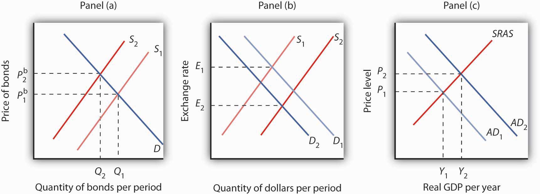
Figure 10.2 "Bond Prices and Macroeconomic Activity" shows how an event in the bond market can stimulate changes in the economy’s output and price level. In Panel (a), an increase in demand for bonds raises bond prices. Interest rates thus fall. Lower interest rates increase the quantity of investment demanded, shifting the aggregate demand curve to the right, from AD1 to AD2 in Panel (b). Real GDP rises from Y1 to Y2; the price level rises from P1 to P2. In Panel (c), an increase in the supply of bonds pushes bond prices down. Interest rates rise. The quantity of investment is likely to fall, shifting aggregate demand to the left, from AD1 to AD2 in Panel (d). Output and the price level fall from Y1 to Y2 and from P1 to P2, respectively. Assuming other determinants of aggregate demand remain unchanged, higher interest rates will tend to reduce aggregate demand and lower interest rates will tend to increase aggregate demand.
Figure 10.2 Bond Prices and Macroeconomic Activity
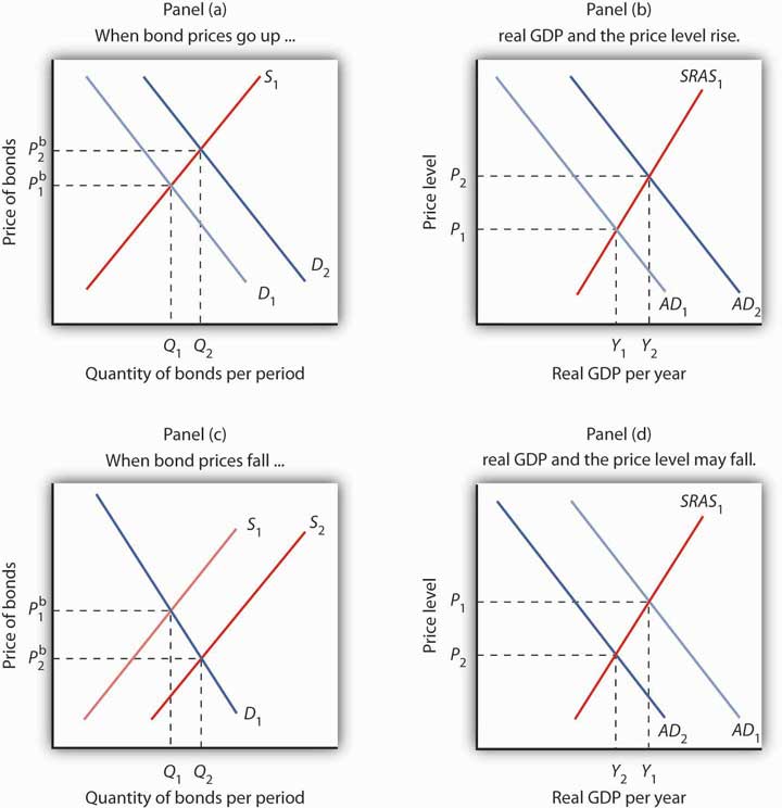
An increase in the demand for bonds to D2 in Panel (a) raises the price of bonds to Pb2, which lowers interest rates and boosts investment. That increases aggregate demand to AD2 in Panel (b); real GDP rises to Y2 and the price level rises to P2.
An increase in the supply of bonds to S2 lowers bond prices to Pb2 in Panel (c) and raises interest rates. The higher interest rate, taken by itself, is likely to cause a reduction in investment and aggregate demand. AD1 falls to AD2, real GDP falls to Y2, and the price level falls to P2 in Panel (d).
In thinking about the impact of changes in interest rates on aggregate demand, we must remember that some events that change aggregate demand can affect interest rates. We will examine those events in subsequent chapters. Our focus in this chapter is on the way in which events that originate in financial markets affect aggregate demand.
Another financial market that influences macroeconomic variables is the foreign exchange marketA market in which currencies of different countries are traded for one another., a market in which currencies of different countries are traded for one another. Since changes in exports and imports affect aggregate demand and thus real GDP and the price level, the market in which currencies are traded has tremendous importance in the economy.
Foreigners who want to purchase goods and services or assets in the United States must typically pay for them with dollars. United States purchasers of foreign goods must generally make the purchase in a foreign currency. An Egyptian family, for example, exchanges Egyptian pounds for dollars in order to pay for admission to Disney World. A German financial investor purchases dollars to buy U.S. government bonds. A family from the United States visiting India, on the other hand, needs to obtain Indian rupees in order to make purchases there. A U.S. bank wanting to purchase assets in Mexico City first purchases pesos. These transactions are accomplished in the foreign exchange market.
The foreign exchange market is not a single location in which currencies are traded. The term refers instead to the entire array of institutions through which people buy and sell currencies. It includes a hotel desk clerk who provides currency exchange as a service to hotel guests, brokers who arrange currency exchanges worth billions of dollars, and governments and central banks that exchange currencies. Major currency dealers are linked by computers so that they can track currency exchanges all over the world.
A country’s exchange rate is the price of its currency in terms of another currency or currencies. On December 12, 2008, for example, the dollar traded for 91.13 Japanese yen, 0.75 euros, 10.11 South African rands, and 13.51 Mexican pesos. There are as many exchange rates for the dollar as there are countries whose currencies exchange for the dollar—roughly 200 of them.
Economists summarize the movement of exchange rates with a trade-weighted exchange rateAn index of exchange rates., which is an index of exchange rates. To calculate a trade-weighted exchange rate index for the U.S. dollar, we select a group of countries, weight the price of the dollar in each country’s currency by the amount of trade between that country and the United States, and then report the price of the dollar based on that trade-weighted average. Because trade-weighted exchange rates are so widely used in reporting currency values, they are often referred to as exchange rates themselves. We will follow that convention in this text.
The rates at which most currencies exchange for one another are determined by demand and supply. How does the model of demand and supply operate in the foreign exchange market?
The demand curve for dollars relates the number of dollars buyers want to buy in any period to the exchange rate. An increase in the exchange rate means it takes more foreign currency to buy a dollar. A higher exchange rate, in turn, makes U.S. goods and services more expensive for foreign buyers and reduces the quantity they will demand. That is likely to reduce the quantity of dollars they demand. Foreigners thus will demand fewer dollars as the price of the dollar—the exchange rate—rises. Consequently, the demand curve for dollars is downward sloping, as in Figure 10.3 "Determining an Exchange Rate".
Figure 10.3 Determining an Exchange Rate
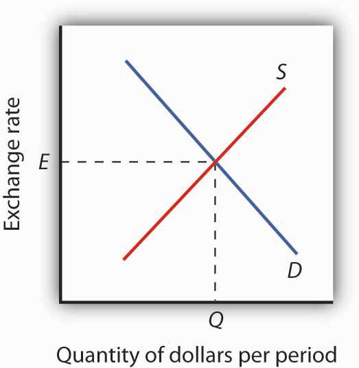
The equilibrium exchange rate is the rate at which the quantity of dollars demanded equals the quantity supplied. Here, equilibrium occurs at exchange rate E, at which Q dollars are exchanged per period.
The supply curve for dollars emerges from a similar process. When people and firms in the United States purchase goods, services, or assets in foreign countries, they must purchase the currency of those countries first. They supply dollars in exchange for foreign currency. The supply of dollars on the foreign exchange market thus reflects the degree to which people in the United States are buying foreign money at various exchange rates. A higher exchange rate means that a dollar trades for more foreign currency. In effect, the higher rate makes foreign goods and services cheaper to U.S. buyers, so U.S. consumers will purchase more foreign goods and services. People will thus supply more dollars at a higher exchange rate; we expect the supply curve for dollars to be upward sloping, as suggested in Figure 10.3 "Determining an Exchange Rate".
In addition to private individuals and firms that participate in the foreign exchange market, most governments participate as well. A government might seek to lower its exchange rate by selling its currency; it might seek to raise the rate by buying its currency. Although governments often participate in foreign exchange markets, they generally represent a very small share of these markets. The most important traders are private buyers and sellers of currencies.
People purchase a country’s currency for two quite different reasons: to purchase goods or services in that country, or to purchase the assets of that country—its money, its capital, its stocks, its bonds, or its real estate. Both of these motives must be considered to understand why demand and supply in the foreign exchange market may change.
One thing that can cause the price of the dollar to rise, for example, is a reduction in bond prices in American markets. Figure 10.4 "Shifts in Demand and Supply for Dollars on the Foreign Exchange Market" illustrates the effect of this change. Suppose the supply of bonds in the U.S. bond market increases from S1 to S2 in Panel (a). Bond prices will drop. Lower bond prices mean higher interest rates. Foreign financial investors, attracted by the opportunity to earn higher returns in the United States, will increase their demand for dollars on the foreign exchange market in order to purchase U.S. bonds. Panel (b) shows that the demand curve for dollars shifts from D1 to D2. Simultaneously, U.S. financial investors, attracted by the higher interest rates at home, become less likely to make financial investments abroad and thus supply fewer dollars to exchange markets. The fall in the price of U.S. bonds shifts the supply curve for dollars on the foreign exchange market from S1 to S2, and the exchange rate rises from E1 to E2.
Figure 10.4 Shifts in Demand and Supply for Dollars on the Foreign Exchange Market
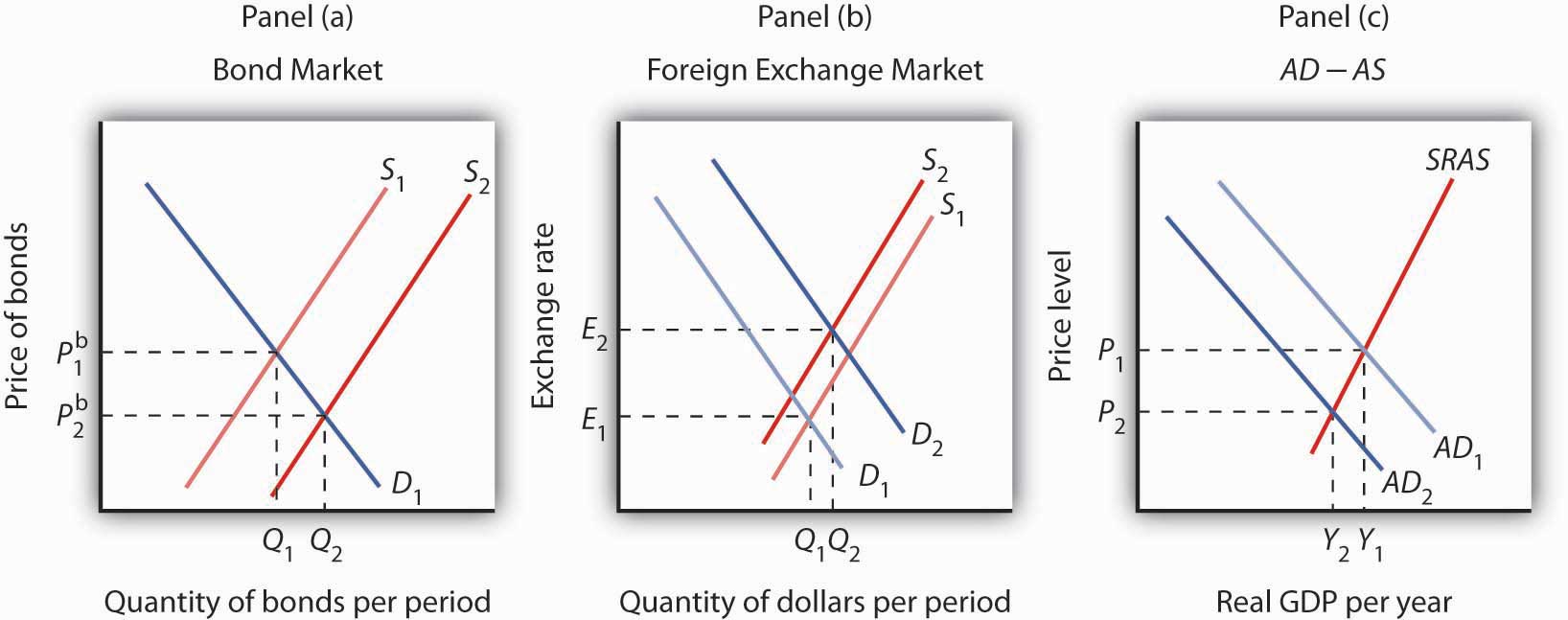
In Panel (a), an increase in the supply of bonds lowers bond prices to Pb2 (and thus raises interest rates). Higher interest rates boost the demand and reduce the supply for dollars, increasing the exchange rate in Panel (b) to E2. These developments in the bond and foreign exchange markets are likely to lead to a reduction in net exports and in investment, reducing aggregate demand from AD1 to AD2 in Panel (c). The price level in the economy falls to P2, and real GDP falls from Y1 to Y2.
The higher exchange rate makes U.S. goods and services more expensive to foreigners, so it reduces exports. It makes foreign goods cheaper for U.S. buyers, so it increases imports. Net exports thus fall, reducing aggregate demand. Panel (c) shows that output falls from Y1 to Y2; the price level falls from P1 to P2. This development in the foreign exchange market reinforces the impact of higher interest rates we observed in Figure 10.2 "Bond Prices and Macroeconomic Activity", Panels (c) and (d). They not only reduce investment—they reduce net exports as well.
Suppose the supply of bonds in the U.S. market decreases. Show and explain the effects on the bond and foreign exchange markets. Use the aggregate demand/aggregate supply framework to show and explain the effects on investment, net exports, real GDP, and the price level.
In October 2011, bond fund manager Bill Gross sent out an extraordinary open letter titled “Mea Culpa.” He was taking the blame for the poor performance of Pimco Total Return Bond Fund, the huge fund he manages. After years of stellar performance, what had gone wrong?
Earlier in 2011, Mr. Gross announced that he would avoid U.S. Treasury bonds. He assumed that as the U.S. and other countries’ economies recovered, interest rates would begin to rise and, hence, U.S. bond prices would fall. When Mr. Gross pulled out of U.S. Treasuries, he used some of the cash to buy other types of debt, such as that of emerging markets. He also held onto some cash. He warned others to shun Treasuries as well.
However, as the financial situation in Europe weakened over worries about government debt in various European countries—starting with Greece and then spilling over to Portugal, Spain, Italy, and others—investors around the world flocked toward Treasuries, pushing Treasury bond prices up. It was a rally that Mr. Gross’s customers missed.
From where did the financial investors get the funds to buy Treasuries? In part, these funds were obtained from some of the same types of bonds that were then in the Pimco fund portfolio. As a result, the prices of bonds in the Pimco fund fell.
In the letter, Mr. Gross wrote, “The simple fact is that the portfolio at midyear was positioned for what we call a ‘New Normal’ developed world economy—2% real growth and 2% inflation. When growth estimates quickly changed it was obvious that I had misjudged the fly ball: E-CF or for nonbaseball aficionados—error centerfield.” In the fall of 2011, he shifted gears and began buying U.S. Treasuries, assuming that a weak global economy would keep interest rates low. He was foiled again, as interest rates started to rise a bit.
In the end, 2011 turned out to be a bad year for the fund, ranking poorly compared to its peers. But after many successful years, it retained its five-star rating by Morningstar in 2012. We must wait to see whether Mr. Gross will get his groove back. In the letter, he concluded, “There is no ‘quit’ in me or anyone else on the Pimco premises. The early morning and even midnight hours have gone up, not down, to match the increasing complexity of the global financial markets. The competitive fire burns even hotter. I/we respect our competition but we want to squash them each and every day…”
Source: “Bill Gross Apologizes to Pimco Fund Owners for ‘Bad Year,’” Los Angeles Times, October 14, 2011, online version.
If the supply of bonds decreases from S1 to S2, bond prices will rise from Pb1 to Pb2, as shown in Panel (a). Higher bond prices mean lower interest rates. Lower interest rates in the United States will make financial investments in the United States less attractive to foreigners. As a result, their demand for dollars will decrease from D1 to D2, as shown in Panel (b). Similarly, U.S. financial investors will look abroad for higher returns and thus supply more dollars to foreign exchange markets, shifting the supply curve from S1 to S2. Thus, the exchange rate will decrease. The quantity of investment rises due to the lower interest rates. Net exports rise because the lower exchange rate makes U.S. goods and services more attractive to foreigners, thus increasing exports, and makes foreign goods less attractive to U.S. buyers, thus reducing imports. Increases in investment and net exports imply a rightward shift in the aggregate demand curve from AD1 to AD2. Real GDP and the price level increase.
In this section we will explore the link between money markets, bond markets, and interest rates. We first look at the demand for money. The demand curve for money is derived like any other demand curve, by examining the relationship between the “price” of money (which, we will see, is the interest rate) and the quantity demanded, holding all other determinants unchanged. We then link the demand for money to the concept of money supply developed in the last chapter, to determine the equilibrium rate of interest. In turn, we show how changes in interest rates affect the macroeconomy.
In deciding how much money to hold, people make a choice about how to hold their wealth. How much wealth shall be held as money and how much as other assets? For a given amount of wealth, the answer to this question will depend on the relative costs and benefits of holding money versus other assets. The demand for moneyThe relationship between the quantity of money people want to hold and the factors that determine that quantity. is the relationship between the quantity of money people want to hold and the factors that determine that quantity.
To simplify our analysis, we will assume there are only two ways to hold wealth: as money in a checking account, or as funds in a bond market mutual fund that purchases long-term bonds on behalf of its subscribers. A bond fund is not money. Some money deposits earn interest, but the return on these accounts is generally lower than what could be obtained in a bond fund. The advantage of checking accounts is that they are highly liquid and can thus be spent easily. We will think of the demand for money as a curve that represents the outcomes of choices between the greater liquidity of money deposits and the higher interest rates that can be earned by holding a bond fund. The difference between the interest rates paid on money deposits and the interest return available from bonds is the cost of holding money.
One reason people hold their assets as money is so that they can purchase goods and services. The money held for the purchase of goods and services may be for everyday transactions such as buying groceries or paying the rent, or it may be kept on hand for contingencies such as having the funds available to pay to have the car fixed or to pay for a trip to the doctor.
The transactions demand for moneyMoney people hold to pay for goods and services they anticipate buying. is money people hold to pay for goods and services they anticipate buying. When you carry money in your purse or wallet to buy a movie ticket or maintain a checking account balance so you can purchase groceries later in the month, you are holding the money as part of your transactions demand for money.
The money people hold for contingencies represents their precautionary demand for moneyThe money people hold for contingencies.. Money held for precautionary purposes may include checking account balances kept for possible home repairs or health-care needs. People do not know precisely when the need for such expenditures will occur, but they can prepare for them by holding money so that they’ll have it available when the need arises.
People also hold money for speculative purposes. Bond prices fluctuate constantly. As a result, holders of bonds not only earn interest but experience gains or losses in the value of their assets. Bondholders enjoy gains when bond prices rise and suffer losses when bond prices fall. Because of this, expectations play an important role as a determinant of the demand for bonds. Holding bonds is one alternative to holding money, so these same expectations can affect the demand for money.
John Maynard Keynes, who was an enormously successful speculator in bond markets himself, suggested that bondholders who anticipate a drop in bond prices will try to sell their bonds ahead of the price drop in order to avoid this loss in asset value. Selling a bond means converting it to money. Keynes referred to the speculative demand for moneyThe money held in response to concern that bond prices and the prices of other financial assets might change. as the money held in response to concern that bond prices and the prices of other financial assets might change.
Of course, money is money. One cannot sort through someone’s checking account and locate which funds are held for transactions and which funds are there because the owner of the account is worried about a drop in bond prices or is taking a precaution. We distinguish money held for different motives in order to understand how the quantity of money demanded will be affected by a key determinant of the demand for money: the interest rate.
The quantity of money people hold to pay for transactions and to satisfy precautionary and speculative demand is likely to vary with the interest rates they can earn from alternative assets such as bonds. When interest rates rise relative to the rates that can be earned on money deposits, people hold less money. When interest rates fall, people hold more money. The logic of these conclusions about the money people hold and interest rates depends on the people’s motives for holding money.
The quantity of money households want to hold varies according to their income and the interest rate; different average quantities of money held can satisfy their transactions and precautionary demands for money. To see why, suppose a household earns and spends $3,000 per month. It spends an equal amount of money each day. For a month with 30 days, that is $100 per day. One way the household could manage this spending would be to leave the money in a checking account, which we will assume pays zero interest. The household would thus have $3,000 in the checking account when the month begins, $2,900 at the end of the first day, $1,500 halfway through the month, and zero at the end of the last day of the month. Averaging the daily balances, we find that the quantity of money the household demands equals $1,500. This approach to money management, which we will call the “cash approach,” has the virtue of simplicity, but the household will earn no interest on its funds.
Consider an alternative money management approach that permits the same pattern of spending. At the beginning of the month, the household deposits $1,000 in its checking account and the other $2,000 in a bond fund. Assume the bond fund pays 1% interest per month, or an annual interest rate of 12.7%. After 10 days, the money in the checking account is exhausted, and the household withdraws another $1,000 from the bond fund for the next 10 days. On the 20th day, the final $1,000 from the bond fund goes into the checking account. With this strategy, the household has an average daily balance of $500, which is the quantity of money it demands. Let us call this money management strategy the “bond fund approach.”
Remember that both approaches allow the household to spend $3,000 per month, $100 per day. The cash approach requires a quantity of money demanded of $1,500, while the bond fund approach lowers this quantity to $500.
The bond fund approach generates some interest income. The household has $1,000 in the fund for 10 days (1/3 of a month) and $1,000 for 20 days (2/3 of a month). With an interest rate of 1% per month, the household earns $10 in interest each month ([$1,000 × 0.01 × 1/3] + [$1,000 × 0.01 × 2/3]). The disadvantage of the bond fund, of course, is that it requires more attention—$1,000 must be transferred from the fund twice each month. There may also be fees associated with the transfers.
Of course, the bond fund strategy we have examined here is just one of many. The household could begin each month with $1,500 in the checking account and $1,500 in the bond fund, transferring $1,500 to the checking account midway through the month. This strategy requires one less transfer, but it also generates less interest—$7.50 (= $1,500 × 0.01 × 1/2). With this strategy, the household demands a quantity of money of $750. The household could also maintain a much smaller average quantity of money in its checking account and keep more in its bond fund. For simplicity, we can think of any strategy that involves transferring money in and out of a bond fund or another interest-earning asset as a bond fund strategy.
Which approach should the household use? That is a choice each household must make—it is a question of weighing the interest a bond fund strategy creates against the hassle and possible fees associated with the transfers it requires. Our example does not yield a clear-cut choice for any one household, but we can make some generalizations about its implications.
First, a household is more likely to adopt a bond fund strategy when the interest rate is higher. At low interest rates, a household does not sacrifice much income by pursuing the simpler cash strategy. As the interest rate rises, a bond fund strategy becomes more attractive. That means that the higher the interest rate, the lower the quantity of money demanded.
Second, people are more likely to use a bond fund strategy when the cost of transferring funds is lower. The creation of savings plans, which began in the 1970s and 1980s, that allowed easy transfer of funds between interest-earning assets and checkable deposits tended to reduce the demand for money.
Some money deposits, such as savings accounts and money market deposit accounts, pay interest. In evaluating the choice between holding assets as some form of money or in other forms such as bonds, households will look at the differential between what those funds pay and what they could earn in the bond market. A higher interest rate in the bond market is likely to increase this differential; a lower interest rate will reduce it. An increase in the spread between rates on money deposits and the interest rate in the bond market reduces the quantity of money demanded; a reduction in the spread increases the quantity of money demanded.
Firms, too, must determine how to manage their earnings and expenditures. However, instead of worrying about $3,000 per month, even a relatively small firm may be concerned about $3,000,000 per month. Rather than facing the difference of $10 versus $7.50 in interest earnings used in our household example, this small firm would face a difference of $2,500 per month ($10,000 versus $7,500). For very large firms such as Toyota or AT&T, interest rate differentials among various forms of holding their financial assets translate into millions of dollars per day.
How is the speculative demand for money related to interest rates? When financial investors believe that the prices of bonds and other assets will fall, their speculative demand for money goes up. The speculative demand for money thus depends on expectations about future changes in asset prices. Will this demand also be affected by present interest rates?
If interest rates are low, bond prices are high. It seems likely that if bond prices are high, financial investors will become concerned that bond prices might fall. That suggests that high bond prices—low interest rates—would increase the quantity of money held for speculative purposes. Conversely, if bond prices are already relatively low, it is likely that fewer financial investors will expect them to fall still further. They will hold smaller speculative balances. Economists thus expect that the quantity of money demanded for speculative reasons will vary negatively with the interest rate.
We have seen that the transactions, precautionary, and speculative demands for money vary negatively with the interest rate. Putting those three sources of demand together, we can draw a demand curve for money to show how the interest rate affects the total quantity of money people hold. The demand curve for moneyCurve that shows the quantity of money demanded at each interest rate, all other things unchanged. shows the quantity of money demanded at each interest rate, all other things unchanged. Such a curve is shown in Figure 10.5 "The Demand Curve for Money". An increase in the interest rate reduces the quantity of money demanded. A reduction in the interest rate increases the quantity of money demanded.
Figure 10.5 The Demand Curve for Money
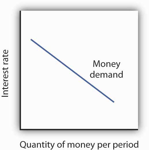
The demand curve for money shows the quantity of money demanded at each interest rate. Its downward slope expresses the negative relationship between the quantity of money demanded and the interest rate.
The relationship between interest rates and the quantity of money demanded is an application of the law of demand. If we think of the alternative to holding money as holding bonds, then the interest rate—or the differential between the interest rate in the bond market and the interest paid on money deposits—represents the price of holding money. As is the case with all goods and services, an increase in price reduces the quantity demanded.
We draw the demand curve for money to show the quantity of money people will hold at each interest rate, all other determinants of money demand unchanged. A change in those “other determinants” will shift the demand for money. Among the most important variables that can shift the demand for money are the level of income and real GDP, the price level, expectations, transfer costs, and preferences.
A household with an income of $10,000 per month is likely to demand a larger quantity of money than a household with an income of $1,000 per month. That relationship suggests that money is a normal good: as income increases, people demand more money at each interest rate, and as income falls, they demand less.
An increase in real GDP increases incomes throughout the economy. The demand for money in the economy is therefore likely to be greater when real GDP is greater.
The higher the price level, the more money is required to purchase a given quantity of goods and services. All other things unchanged, the higher the price level, the greater the demand for money.
The speculative demand for money is based on expectations about bond prices. All other things unchanged, if people expect bond prices to fall, they will increase their demand for money. If they expect bond prices to rise, they will reduce their demand for money.
The expectation that bond prices are about to change actually causes bond prices to change. If people expect bond prices to fall, for example, they will sell their bonds, exchanging them for money. That will shift the supply curve for bonds to the right, thus lowering their price. The importance of expectations in moving markets can lead to a self-fulfilling prophecy.
Expectations about future price levels also affect the demand for money. The expectation of a higher price level means that people expect the money they are holding to fall in value. Given that expectation, they are likely to hold less of it in anticipation of a jump in prices.
Expectations about future price levels play a particularly important role during periods of hyperinflation. If prices rise very rapidly and people expect them to continue rising, people are likely to try to reduce the amount of money they hold, knowing that it will fall in value as it sits in their wallets or their bank accounts. Toward the end of the great German hyperinflation of the early 1920s, prices were doubling as often as three times a day. Under those circumstances, people tried not to hold money even for a few minutes—within the space of eight hours money would lose half its value!
For a given level of expenditures, reducing the quantity of money demanded requires more frequent transfers between nonmoney and money deposits. As the cost of such transfers rises, some consumers will choose to make fewer of them. They will therefore increase the quantity of money they demand. In general, the demand for money will increase as it becomes more expensive to transfer between money and nonmoney accounts. The demand for money will fall if transfer costs decline. In recent years, transfer costs have fallen, leading to a decrease in money demand.
Preferences also play a role in determining the demand for money. Some people place a high value on having a considerable amount of money on hand. For others, this may not be important.
Household attitudes toward risk are another aspect of preferences that affect money demand. As we have seen, bonds pay higher interest rates than money deposits, but holding bonds entails a risk that bond prices might fall. There is also a chance that the issuer of a bond will default, that is, will not pay the amount specified on the bond to bondholders; indeed, bond issuers may end up paying nothing at all. A money deposit, such as a savings deposit, might earn a lower yield, but it is a safe yield. People’s attitudes about the trade-off between risk and yields affect the degree to which they hold their wealth as money. Heightened concerns about risk in the last half of 2008 led many households to increase their demand for money.
Figure 10.6 "An Increase in Money Demand" shows an increase in the demand for money. Such an increase could result from a higher real GDP, a higher price level, a change in expectations, an increase in transfer costs, or a change in preferences.
Figure 10.6 An Increase in Money Demand
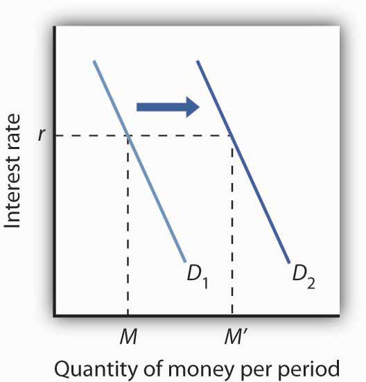
An increase in real GDP, the price level, or transfer costs, for example, will increase the quantity of money demanded at any interest rate r, increasing the demand for money from D1 to D2. The quantity of money demanded at interest rate r rises from M to M′. The reverse of any such events would reduce the quantity of money demanded at every interest rate, shifting the demand curve to the left.
The supply curve of moneyCurve that shows the relationship between the quantity of money supplied and the market interest rate, all other determinants of supply unchanged. shows the relationship between the quantity of money supplied and the market interest rate, all other determinants of supply unchanged. We have learned that the Fed, through its open-market operations, determines the total quantity of reserves in the banking system. We shall assume that banks increase the money supply in fixed proportion to their reserves. Because the quantity of reserves is determined by Federal Reserve policy, we draw the supply curve of money in Figure 10.7 "The Supply Curve of Money" as a vertical line, determined by the Fed’s monetary policies. In drawing the supply curve of money as a vertical line, we are assuming the money supply does not depend on the interest rate. Changing the quantity of reserves and hence the money supply is an example of monetary policy.
Figure 10.7 The Supply Curve of Money
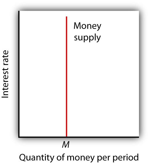
We assume that the quantity of money supplied in the economy is determined as a fixed multiple of the quantity of bank reserves, which is determined by the Fed. The supply curve of money is a vertical line at that quantity.
The money marketThe interaction among institutions through which money is supplied to individuals, firms, and other institutions that demand money. is the interaction among institutions through which money is supplied to individuals, firms, and other institutions that demand money. Money market equilibriumThe interest rate at which the quantity of money demanded is equal to the quantity of money supplied. occurs at the interest rate at which the quantity of money demanded is equal to the quantity of money supplied. Figure 10.8 "Money Market Equilibrium" combines demand and supply curves for money to illustrate equilibrium in the market for money. With a stock of money (M), the equilibrium interest rate is r.
Figure 10.8 Money Market Equilibrium
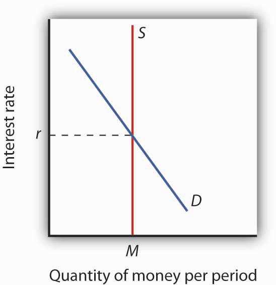
The market for money is in equilibrium if the quantity of money demanded is equal to the quantity of money supplied. Here, equilibrium occurs at interest rate r.
A shift in money demand or supply will lead to a change in the equilibrium interest rate. Let’s look at the effects of such changes on the economy.
Suppose that the money market is initially in equilibrium at r1 with supply curve S and a demand curve D1 as shown in Panel (a) of Figure 10.9 "A Decrease in the Demand for Money". Now suppose that there is a decrease in money demand, all other things unchanged. A decrease in money demand could result from a decrease in the cost of transferring between money and nonmoney deposits, from a change in expectations, or from a change in preferences.In this chapter we are looking only at changes that originate in financial markets to see their impact on aggregate demand and aggregate supply. Changes in the price level and in real GDP also shift the money demand curve, but these changes are the result of changes in aggregate demand or aggregate supply and are considered in more advanced courses in macroeconomics. Panel (a) shows that the money demand curve shifts to the left to D2. We can see that the interest rate will fall to r2. To see why the interest rate falls, we recall that if people want to hold less money, then they will want to hold more bonds. Thus, Panel (b) shows that the demand for bonds increases. The higher price of bonds means lower interest rates; lower interest rates restore equilibrium in the money market.
Figure 10.9 A Decrease in the Demand for Money
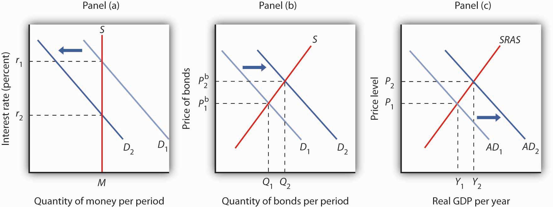
A decrease in the demand for money due to a change in transactions costs, preferences, or expectations, as shown in Panel (a), will be accompanied by an increase in the demand for bonds as shown in Panel (b), and a fall in the interest rate. The fall in the interest rate will cause a rightward shift in the aggregate demand curve from AD1 to AD2, as shown in Panel (c). As a result, real GDP and the price level rise.
Lower interest rates in turn increase the quantity of investment. They also stimulate net exports, as lower interest rates lead to a lower exchange rate. The aggregate demand curve shifts to the right as shown in Panel (c) from AD1 to AD2. Given the short-run aggregate supply curve SRAS, the economy moves to a higher real GDP and a higher price level.
An increase in money demand due to a change in expectations, preferences, or transactions costs that make people want to hold more money at each interest rate will have the opposite effect. The money demand curve will shift to the right and the demand for bonds will shift to the left. The resulting higher interest rate will lead to a lower quantity of investment. Also, higher interest rates will lead to a higher exchange rate and depress net exports. Thus, the aggregate demand curve will shift to the left. All other things unchanged, real GDP and the price level will fall.
Now suppose the market for money is in equilibrium and the Fed changes the money supply. All other things unchanged, how will this change in the money supply affect the equilibrium interest rate and aggregate demand, real GDP, and the price level?
Suppose the Fed conducts open-market operations in which it buys bonds. This is an example of expansionary monetary policy. The impact of Fed bond purchases is illustrated in Panel (a) of Figure 10.10 "An Increase in the Money Supply". The Fed’s purchase of bonds shifts the demand curve for bonds to the right, raising bond prices to Pb2. As we learned, when the Fed buys bonds, the supply of money increases. Panel (b) of Figure 10.10 "An Increase in the Money Supply" shows an economy with a money supply of M, which is in equilibrium at an interest rate of r1. Now suppose the bond purchases by the Fed as shown in Panel (a) result in an increase in the money supply to M′; that policy change shifts the supply curve for money to the right to S2. At the original interest rate r1, people do not wish to hold the newly supplied money; they would prefer to hold nonmoney assets. To reestablish equilibrium in the money market, the interest rate must fall to increase the quantity of money demanded. In the economy shown, the interest rate must fall to r2 to increase the quantity of money demanded to M′.
Figure 10.10 An Increase in the Money Supply
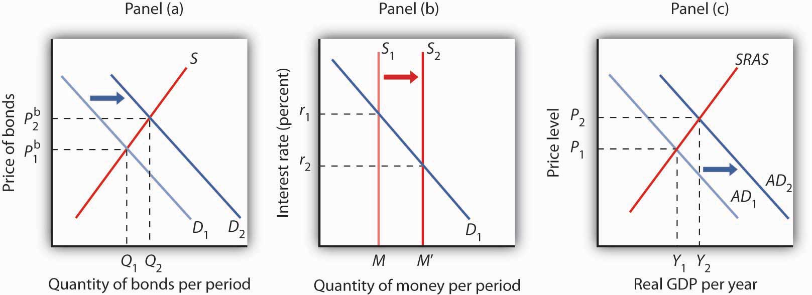
The Fed increases the money supply by buying bonds, increasing the demand for bonds in Panel (a) from D1 to D2 and the price of bonds to Pb2. This corresponds to an increase in the money supply to M′ in Panel (b). The interest rate must fall to r2 to achieve equilibrium. The lower interest rate leads to an increase in investment and net exports, which shifts the aggregate demand curve from AD1 to AD2 in Panel (c). Real GDP and the price level rise.
The reduction in interest rates required to restore equilibrium to the market for money after an increase in the money supply is achieved in the bond market. The increase in bond prices lowers interest rates, which will increase the quantity of money people demand. Lower interest rates will stimulate investment and net exports, via changes in the foreign exchange market, and cause the aggregate demand curve to shift to the right, as shown in Panel (c), from AD1 to AD2. Given the short-run aggregate supply curve SRAS, the economy moves to a higher real GDP and a higher price level.
Open-market operations in which the Fed sells bonds—that is, a contractionary monetary policy—will have the opposite effect. When the Fed sells bonds, the supply curve of bonds shifts to the right and the price of bonds falls. The bond sales lead to a reduction in the money supply, causing the money supply curve to shift to the left and raising the equilibrium interest rate. Higher interest rates lead to a shift in the aggregate demand curve to the left.
As we have seen in looking at both changes in demand for and in supply of money, the process of achieving equilibrium in the money market works in tandem with the achievement of equilibrium in the bond market. The interest rate determined by money market equilibrium is consistent with the interest rate achieved in the bond market.
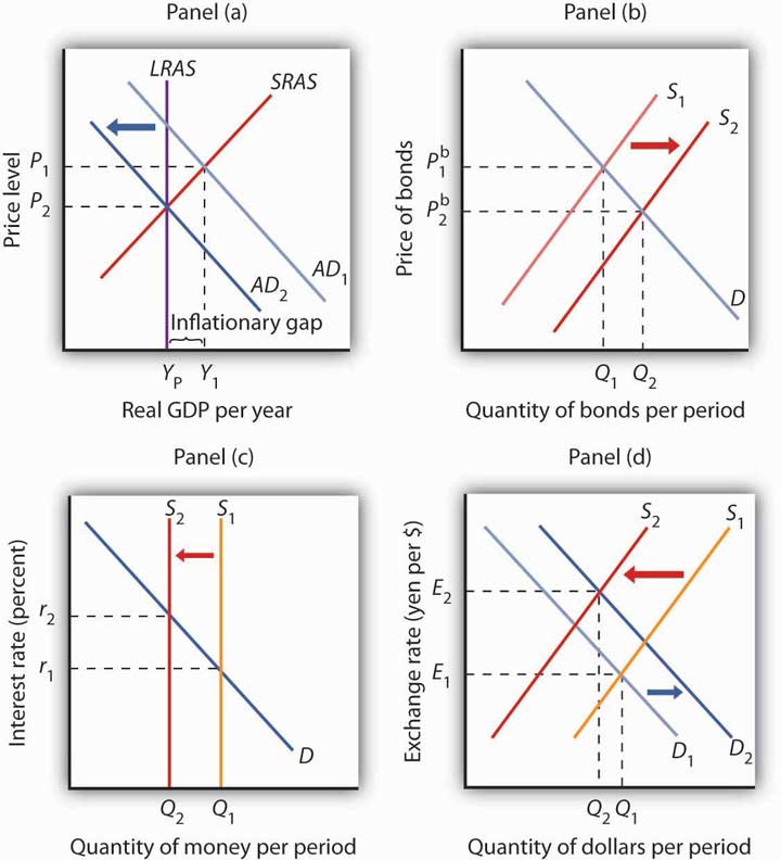
In 2005 the Fed was concerned about the possibility that the United States was moving into an inflationary gap, and it adopted a contractionary monetary policy as a result. Draw a four-panel graph showing this policy and its expected results. In Panel (a), use the model of aggregate demand and aggregate supply to illustrate an economy with an inflationary gap. In Panel (b), show how the Fed’s policy will affect the market for bonds. In Panel (c), show how it will affect the demand for and supply of money. In Panel (d), show how it will affect the exchange rate. Finally, return to Panel (a) and incorporate these developments into your analysis of aggregate demand and aggregate supply, and show how the Fed’s policy will affect real GDP and the price level in the short run.

The models of the money and bond markets presented in this chapter suggest that the Fed can control the interest rate by deciding on a money supply that would lead to the desired equilibrium interest rate in the money market. Yet, Fed policy announcements typically focus on what it wants the federal funds rate to be with scant attention to the money supply. Whereas throughout the 1990s, the Fed would announce a target federal funds rate and also indicate an expected change in the money supply, in 2000, when legislation requiring it to do so expired, it abandoned the practice of setting money supply targets.
Why the shift? The factors that have made focusing on the money supply as a policy target difficult for the past 25 years are first banking deregulation in the 1980s followed by financial innovations associated with technological changes—in particular the maturation of electronic payment and transfer mechanisms—thereafter.
Before the 1980s, M1 was a fairly reliable measure of the money people held, primarily for transactions. To buy things, one used cash, checks written on demand deposits, or traveler’s checks. The Fed could thus use reliable estimates of the money demand curve to predict what the money supply would need to be in order to bring about a certain interest rate in the money market.
Legislation in the early 1980s allowed for money market deposit accounts (MMDAs), which are essentially interest-bearing savings accounts on which checks can be written. MMDAs are part of M2. Shortly after, other forms of payments for transactions developed or became more common. For example, credit and debit card use has mushroomed (from $10.8 billion in 1990 to $30 billion in 2000), and people can pay their credit card bills, electronically or with paper checks, from accounts that are part of either M1 or M2. Another innovation of the last 20 years is the automatic transfer service (ATS) that allows consumers to move money between checking and savings accounts at an ATM machine, or online, or through prearranged agreements with their financial institutions. While we take these methods of payment for granted today, they did not exist before 1980 because of restrictive banking legislation and the lack of technological know-how. Indeed, before 1980, being able to pay bills from accounts that earned interest was unheard of.
Further blurring the lines between M1 and M2 has been the development and growing popularity of what are called retail sweep programs. Since 1994, banks have been using retail-sweeping software to dynamically reclassify balances as either checking account balances (part of M1) or MMDAs (part of M2). They do this to avoid reserve requirements on checking accounts. The software not only moves the funds but also ensures that the bank does not exceed the legal limit of six reclassifications in any month. In the last 10 years these retail sweeps rose from zero to nearly the size of M1 itself!
Such changes in the ways people pay for transactions and banks do their business have led economists to think about new definitions of money that would better track what is actually used for the purposes behind the money demand curve. One notion is called MZM, which stands for “money zero maturity.” The idea behind MZM is that people can easily use any deposits that do not have specified maturity terms to pay for transactions, as these accounts are quite liquid, regardless of what classification of money they fall into. Some research shows that using MZM allows for a stable picture of the money market. Until more agreement has been reached, though, we should expect the Fed to continue to downplay the role of the money supply in its policy deliberations and to continue to announce its intentions in terms of the federal funds rate.
Source: Pedre Teles and Ruilin Zhou, “A Stable Money Demand: Looking for the Right Monetary Aggregate,” Federal Reserve Bank of Chicago Economic Perspectives 29 (First Quarter, 2005): 50–59.
In Panel (a), with the aggregate demand curve AD1, short-run aggregate supply curve SRAS, and long-run aggregate supply curve LRAS, the economy has an inflationary gap of Y1 − YP. The contractionary monetary policy means that the Fed sells bonds—a rightward shift of the bond supply curve in Panel (b), which decreases the money supply—as shown by a leftward shift in the money supply curve in Panel (c). In Panel (b), we see that the price of bonds falls, and in Panel (c) that the interest rate rises. A higher interest rate will reduce the quantity of investment demanded. The higher interest rate also leads to a higher exchange rate, as shown in Panel (d), as the demand for dollars increases and the supply decreases. The higher exchange rate will lead to a decrease in net exports. As a result of these changes in financial markets, the aggregate demand curve shifts to the left to AD2 in Panel (a). If all goes according to plan (and we will learn in the next chapter that it may not!), the new aggregate demand curve will intersect SRAS and LRAS at YP.
We began this chapter by looking at bond and foreign exchange markets and showing how each is related to the level of real GDP and the price level. Bonds represent the obligation of the seller to repay the buyer the face value by the maturity date; their interest rate is determined by the demand and supply for bonds. An increase in bond prices means a drop in interest rates. A reduction in bond prices means interest rates have risen. The price of the dollar is determined in foreign exchange markets by the demand and supply for dollars.
We then saw how the money market works. The quantity of money demanded varies negatively with the interest rate. Factors that cause the demand curve for money to shift include changes in real GDP, the price level, expectations, the cost of transferring funds between money and nonmoney accounts, and preferences, especially preferences concerning risk. Equilibrium in the market for money is achieved at the interest rate at which the quantity of money demanded equals the quantity of money supplied. We assumed that the supply of money is determined by the Fed. An increase in money demand raises the equilibrium interest rate, and a decrease in money demand lowers the equilibrium interest rate. An increase in the money supply lowers the equilibrium interest rate; a reduction in the money supply raises the equilibrium interest rate.
How would each of the following affect the demand for money?
Compute the rate of interest associated with each of these bonds that matures in one year:
| Face Value | Selling Price | |
|---|---|---|
a. |
$100 |
$80 |
b. |
$100 |
$90 |
c. |
$100 |
$95 |
d. |
$200 |
$180 |
e. |
$200 |
$190 |
f. |
$200 |
$195 |
g. |
Describe the relationship between the selling price of a bond and the interest rate. |
|
Suppose that the demand and supply schedules for bonds that have a face value of $100 and a maturity date one year hence are as follows:
| Price ($) | Quantity Demanded | Quantity Supplied |
|---|---|---|
| 100 | 0 | 600 |
| 95 | 100 | 500 |
| 90 | 200 | 400 |
| 85 | 300 | 300 |
| 80 | 400 | 200 |
| 75 | 500 | 100 |
| 70 | 600 | 0 |
Compute the dollar price of a German car that sells for 40,000 euros at each of the following exchange rates:
Consider the euro-zone of the European Union and Japan. The demand and supply curves for euros are given by the following table (prices for the euro are given in Japanese yen; quantities of euros are in millions):
| Price (in Euros) | Euros Demanded | Euros Supplied |
|---|---|---|
| 75 | 0 | 600 |
| 70 | 100 | 500 |
| 65 | 200 | 400 |
| 60 | 300 | 300 |
| 55 | 400 | 200 |
| 50 | 500 | 100 |
| 45 | 600 | 0 |
Suppose you earn $6,000 per month and spend $200 in each of the month’s 30 days. Compute your average quantity of money demanded if:
Suppose the quantity demanded of money at an interest rate of 5% is $2 billion per day, at an interest rate of 3% is $3 billion per day, and at an interest rate of 1% is $4 billion per day. Suppose the money supply is $3 billion per day.


