It all began September 17, 2011, with a march by thousands of demonstrators unhappy with all sorts of things about the United States—the distribution of income, with rallying cries on behalf of the 99%; “greed” on Wall Street; the bailout of many banks; capitalism in general; and a variety of other perceived ills, from hostility to certain nonfinancial companies such as Walmart and Starbucks to calls for the United States to pull out of military operations around the world and to abolish the Federal Reserve Bank. The symbol of the movement became the occupation of a small park in the neighborhood of Wall Street—Zuccotti Park. Two months later, the park continued to be jammed with demonstrators using it as a campground, after which New York City Mayor Michael Bloomberg shut it down as a place for overnight lodging.
Well before then, the “Occupy Wall Street” movement had become a national phenomenon and then an international phenomenon. The Economist in mid-October reported demonstrations in more than 900 cities and in more than 80 countries. The demonstrators generally rejected the entire concept of making specific demands, preferring instead to protest in support of an ill-defined, but clearly compelling, message—whatever that message might have been.
Who were the demonstrators? Douglas Schoen, who once worked as a pollster for President Bill Clinton, had his survey firm interview about 200 protesters occupying Zuccotti Park in mid-October of 2011 about their views. According to Schoen's survey, the Zuccotti Park demonstrators were committed to a radical redistribution of income and sharp increases in government regulation of the economy, with 98% of them supporting civil disobedience to further their aims and 31% advocating violent measures to achieve their goals. A Pew survey at about the same time found Americans divided in their opinion about the “Occupy Wall Street” movement, with nearly 40% in support and about 35% opposed. At the same time, support and opposition for the Tea Party were running 32% in favor and 44% opposed.“Not Quite Together,” Economist, October 22, 2011; Douglas Schoen, “Polling the Occupy Wall Street Crowd,” Wall Street Journal Online, October 18, 2011; “Public Divided Over Occupy Wall Street Movement,” Pew Charitable Trust Pew Research Center for the People & the Press, http://www.people-press.org/2011/10/24/public-divided-over-occupy-wall-street-movement/.
Whatever the makeup of the groups demonstrating throughout the world, they clearly brought the issues examined in this chapter—poverty, discrimination, and the distribution of income—to the forefront of public attention. It was not obvious why inequality and related complaints had suddenly become an important issue. As we will see on this chapter, inequality in the U.S. distribution of income had begun increasing in 1967; it has continued to rise ever since.
At about the same time as the movement was in the news, the poverty rate in the United States reached its highest level since 1993. The number of people below the U.S. poverty line in 2010—an annual income of $22,314 for a family of four—rose to 15.1% of the population. The number of people considered to be below the poverty level rose to 46.2 million, the highest number ever recorded in the history of the United States. Those statistics came more than four decades after President Lyndon B. Johnson stood before the Congress of the United States to make his first State of the Union address in 1964 to declare a new kind of war, a War on Poverty. “This administration today here and now declares unconditional war on poverty in America,” the President said. “Our aim is not only to relieve the symptoms of poverty but to cure it; and, above, all, to prevent it.” In the United States that year, 35.1 million people, about 22% of the population, were, by the official definition, poor.
The President’s plan included stepped-up federal aid to low-income people, an expanded health-care program for the poor, new housing subsidies, expanded federal aid to education, and job training programs. The proposal became law later that same year. More than four decades and trillions of dollars in federal antipoverty spending later, the nation seems to have made little progress toward the President’s goal.
In this chapter, we shall also explore the problem of discrimination. Being at the lower end of the income distribution and being poor are more prevalent among racial minorities and among women than among white males. To a degree, this situation may reflect discrimination. We shall investigate the economics of discrimination and its consequences for the victims and for the economy. We shall also assess efforts by the public sector to eliminate discrimination.
Questions of fairness often accompany discussions of income inequality, poverty, and discrimination. Answering them ultimately involves value judgments; they are normative questions, not positive ones. You must decide for yourself if a particular distribution of income is fair or if society has made adequate progress toward reducing poverty or discrimination. The material in this chapter will not answer those questions for you; rather, in order for you to have a more informed basis for making your own value judgments, it will shed light on what economists have learned about these issues through study and testing of hypotheses.
Income inequality in the United States has soared in the last half century. According to the Congressional Budget Office, between 1979 and 2007, real average household income—taking into account government transfers and federal taxes—rose 62%. For the top 1% of the population, it grew 275%. For others in the top 20% of the population, it grew 65%. For the 60% of the population in the middle, it grew a bit under 40% and for the 20% of the population at the lowest end of the income distribution, it grew about 18%.Congressional Budget Office, “Trends in the Distribution of Household Income Between 1979 and 2007,” October 2011, http://www.cbo.gov/ftpdocs/124xx/doc12485/10-25-HouseholdIncome.pdf.
Increasingly, education is the key to a better material life. The gap between the average annual incomes of high school graduates and those with a bachelor’s degree increased substantially over the last half century. A recent study undertaken at the Georgetown University Center on Education and the Workforce concluded that people with a bachelor’s degree earn 84% more over a lifetime than do people who are high school graduates only. That college premium is up from 75% in 1999.Anthony P. Carnevale, Stephen J. Rose, and Ban Cheah, The College Payoff: Education, Occupation, and Lifetime Earnings, Georgetown University Center on Education and the Workforce: 2011, http://cew.georgetown.edu/collegepayoff. Moreover, education is not an equal opportunity employer. A student from a family in the upper end of the income distribution is much more likely to get a college degree than a student whose family is in the lower end of the income distribution.
That inequality perpetuates itself. College graduates marry other college graduates and earn higher incomes. Those who do not go to college earn lower incomes. Some may have children out of wedlock—an almost sure route to poverty. That does not, of course, mean that young people who go to college are assured high incomes while those who do not are certain to experience poverty, but the odds certainly push in that direction.
We shall learn in this section how the degree of inequality can be measured. We shall examine the sources of rising inequality and consider what policy measures, if any, are suggested. In this section on inequality we are essentially focusing the way the economic pie is shared, while setting aside the important fact that the size of the economic pie has certainly grown over time.
We have seen that the income distribution has become more unequal. This section describes a graphical approach to measuring the equality, or inequality, of the distribution of income.
The primary evidence of growing inequality is provided by census data. Households are asked to report their income, and they are ranked from the household with the lowest income to the household with the highest income. The Census Bureau then reports the percentage of total income earned by those households ranked among the bottom 20%, the next 20%, and so on, up to the top 20%. Each 20% of households is called a quintile. The bureau also reports the share of income going to the top 5% of households.
Income distribution data can be presented graphically using a Lorenz curveA curve that shows cumulative shares of income received by individuals or groups., a curve that shows cumulative shares of income received by individuals or groups. It was developed by economist Max O. Lorenz in 1905. To plot the curve, we begin with the lowest quintile and mark a point to show the percentage of total income those households received. We then add the next quintile and its share and mark a point to show the share of the lowest 40% of households. Then, we add the third quintile, and then the fourth. Since the share of income received by all the quintiles will be 100%, the last point on the curve always shows that 100% of households receive 100% of the income.
If every household in the United States received the same income, the Lorenz curve would coincide with the 45-degree line drawn in Figure 18.1 "The Distribution of U.S. Income, 1968 and 2010". The bottom 20% of households would receive 20% of income; the bottom 40% would receive 40%, and so on. If the distribution of income were completely unequal, with one household receiving all the income and the rest zero, then the Lorenz curve would be shaped like a backward L, with a horizontal line across the bottom of the graph at 0% income and a vertical line up the right-hand side. The vertical line would show, as always, that 100% of families still receive 100% of income. Actual Lorenz curves lie between these extremes. The closer a Lorenz curve lies to the 45-degree line, the more equal the distribution. The more bowed out the curve, the less equal the distribution. We see in Figure 18.1 "The Distribution of U.S. Income, 1968 and 2010" that the Lorenz curve for the United States became more bowed out between 1968 and 2010.
Figure 18.1 The Distribution of U.S. Income, 1968 and 2010
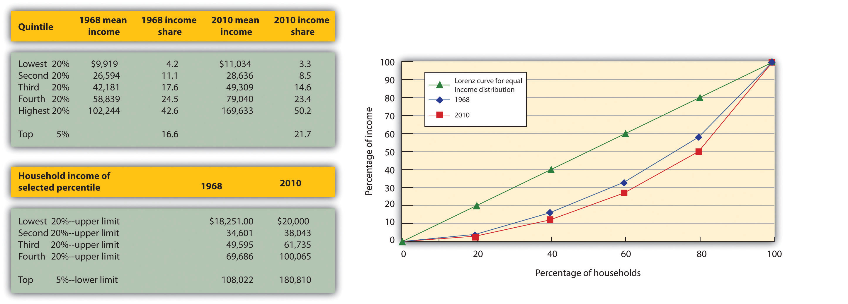
The distribution of income among households in the United States became more unequal from 1968 to 2010. The shares of income received by each of the first four quintiles fell, while the share received by the top 20% rose sharply. The Lorenz curve for 2010 was more bowed out than was the curve for 1968. (Mean income adjusted for inflation and reported in 2010 dollars; percentages do not sum to 100% due to rounding.)
Sources: Carmen DeNavas-Walt, Bernadette D. Proctor, and Jessica C. Smith, U.S. Census Bureau, Current Population Reports, P60-239, Income, Poverty, and Health Insurance Coverage in the United States: 2010, U.S. Government Printing Office, Washington, DC, 2011, Table A-3; U.S. Census Bureau, Current Population Survey, 2010 Annual Social and Economic Supplement, Table HINC-05.
The degree of inequality is often measured with a Gini coefficientA measure of inequality expressed as the ratio of the area between the Lorenz curve and a 45° line and the total area under the 45° line., the ratio between the Lorenz curve and the 45° line and the total area under the 45° line. The smaller the Gini coefficient, the more equal the income distribution. Larger Gini coefficients mean more unequal distributions. The Census Bureau reported that the Gini coefficient was 0.359 in 1968 and 0.457 in 2010.Carmen DeNavas-Walt, Bernadette D. Proctor, and Jessica C. Smith, U.S. Census Bureau, Current Population Reports, P60-239, Income, Poverty, and Health Insurance Coverage in the United States: 2010, U.S. Government Printing Office, Washington, DC, 2011.
When we speak of the bottom 20% or the middle 20% of families, we are not speaking of a static group. Some families who are in the bottom quintile one year move up to higher quintiles in subsequent years; some families move down. Because people move up and down the distribution, we get a quite different picture of income change when we look at the incomes of a fixed set of persons over time rather than comparing average incomes for a particular quintile at a particular point in time, as was done in Figure 18.1 "The Distribution of U.S. Income, 1968 and 2010".
Addressing the question of mobility requires that researchers follow a specific group of families over a long period of time. Since 1968, the Panel Survey of Income Dynamics (PSID) at the University of Michigan has followed more than 5,000 families and their descendents. The effort has produced a much deeper understanding of changes in income inequality than it is possible to obtain from census data, which simply take a snapshot of incomes at a particular time.
Based on the University of Michigan’s data, Federal Reserve Bank of Boston economist Katharine Bradbury compared mobility over the decades through 2005. She concluded that on most mobility measures, family income mobility was significantly lower in the 1990s and early 2000s than in earlier periods. Moreover, when families move out of a quintile, they move less. Finally, she notes that for the recent decades moving across quintiles has become harder to achieve precisely because of the increased income inequality.Katharine Bradbury, “Trends in U.S. Family Income Mobility, 1969–2006,” Federal Reserve Bank of Boston Working Paper no. 11-10, October 20, 2011.
Everyone agrees that the distribution of income in the United States generally became more equal during the first two decades after World War II and that it has become more unequal since 1968. While some people conclude that this increase in inequality suggests the latter period was unfair, others want to know why the distribution changed. We shall examine some of the explanations.
Clearly, an important source of rising inequality since 1968 has been the sharp increase in the number of families headed by women. In 2010, the median income of families headed by married couples was 2.5 times that of families headed by women without a spouse. The percentage of families headed by women with no spouse present has nearly doubled since 1968 and is thus contributing to increased inequality across households.
Technological change has affected the demand for labor. One of the most dramatic changes since the late 1970s has been an increase in the demand for skilled labor and a reduction in the demand for unskilled labor.
The result has been an increase in the gap between the wages of skilled and unskilled workers. That has produced a widening gap between college- and high-school-trained workers.
Technological change has meant the integration of computers into virtually every aspect of production. And that has increased the demand for workers with the knowledge to put new methods to work—and to adapt to the even more dramatic changes in production likely to come. At the same time, the demand for workers who do not have that knowledge has fallen.
Along with new technologies that require greater technical expertise, firms are adopting new management styles that require stronger communication skills. The use of production teams, for example, shifts decision-making authority to small groups of assembly-line workers. That means those workers need more than the manual dexterity that was required of them in the past. They need strong communication skills. They must write effectively, speak effectively, and interact effectively with other workers. Workers who cannot do so simply are not in demand to the degree they once were.
The “intellectual wage gap” seems likely to widen as we move even further into the twenty-first century. That is likely to lead to an even higher degree of inequality and to pose a challenge to public policy for decades to come. Increasing education and training could lead to reductions in inequality. Indeed, individuals seem to have already begun to respond to this changing market situation, since the percentage who graduate from high school and college is rising.
Did tax policy contribute to rising inequality over the past four decades? The tax changes most often cited in the fairness debate are the Reagan tax cuts introduced in 1981 and the Bush tax cuts introduced in 2001, 2002, and 2003.
An analysis of the Bush tax cuts by the Tax Foundation combines the three Bush tax cuts and assumes they occurred in 2003. Table 18.1 "Income Tax Liability Before and After the Bush Tax Cuts" gives the share of total income tax liability for each quintile before and after the Bush tax cuts. It also gives the share of the Bush tax cuts received by each quintile.
Table 18.1 Income Tax Liability Before and After the Bush Tax Cuts
| Quintile | Share of income tax liability before tax cuts | Share of income tax liability after tax cuts | Share of total tax relief |
|---|---|---|---|
| First quintile | 0.5% | 0.3% | 1.2% |
| Second quintile | 2.3% | 1.9% | 4.2% |
| Third quintile | 5.9% | 5.2% | 9.4% |
| Fourth quintile | 12.6% | 11.6% | 17.5% |
| Top quintile | 78.7% | 81.0% | 67.7% |
The share of total tax relief received by the first four quintiles was modest, while those in the top quintile received more than two-thirds of the total benefits of the three tax cuts. However, the share of income taxes paid by each of the first four quintiles fell as a result of the tax cuts, while the share paid by the top quintile rose.
Source: William Ahean, “Comparing the Kennedy, Reagan, and Bush Tax Cuts,” Tax Foundation Fiscal Facts, August 24, 2004.
Tax cuts under George W. Bush were widely criticized as being tilted unfairly toward the rich. And certainly, Table 18.1 "Income Tax Liability Before and After the Bush Tax Cuts" shows that the share of total tax relief received by the first four quintiles was modest, while those in the top quintile garnered more than two-thirds of the total benefits of the three tax cuts. Looking at the second and third columns of the table, however, gives a different perspective. The share of income taxes paid by each of the first four quintiles fell as a result of the tax cuts, while the share paid by the top quintile rose. Further, we see that each of the first four quintiles paid a very small share of income taxes before and after the tax cuts, while those in the top quintile ended up shouldering more than 80% of the total income tax burden. We saw in Figure 18.1 "The Distribution of U.S. Income, 1968 and 2010" that those in the top quintile received just over half of total income. After the Bush tax cuts, they paid 81% of income taxes. Others are quick to point out that those same tax cuts were accompanied by reductions in expenditures for some social service programs designed to help lower income families. Still others point out that the tax cuts contributed to an increase in the federal deficit and, therefore, are likely to have distributional effects over many years and across several generations. Whether these changes increased or decreased fairness in the society is ultimately a normative question.
The method by which the Census Bureau computes income shares has been challenged by some observers. For example, quintiles of households do not contain the same number of people. Rea Hederman of the Heritage Foundation, a conservative think tank, notes that the top 20% of households contains about 25% of the population. Starting in 2006, the Census Bureau report began calculating a measure called “equivalence-adjusted income” to take into account family size. The Gini coefficient for 2010 using this adjustment fell slightly from 0.469 to 0.457. The trend over time in the two Gini coefficients is similar. Two other flaws pointed out by Mr. Hederman are that taxes and benefits from noncash programs that help the poor are not included. While some Census studies attempt to take these into account and report lower inequality, other studies do not receive as much attention as the main Census annual report.Rea S. Hederman, Jr., “Census Report Adds New Twist to Income Inequality Data,” Heritage Foundation, Policy Research and Analysis, No. 1592, August 29, 2007.
Even studies that look at incomes over a decade may not capture lifetime income. For example, people in retirement may have a low income but their consumption may be bolstered by drawing on their savings. Younger people may be borrowing to go to school, buy a house, or for other things. The annual income approach of the Census data does not capture this and even the ten-year look in the mobility study mentioned above is too short a period.
This suggests that more precise measurements may provide more insight into explaining inequality.
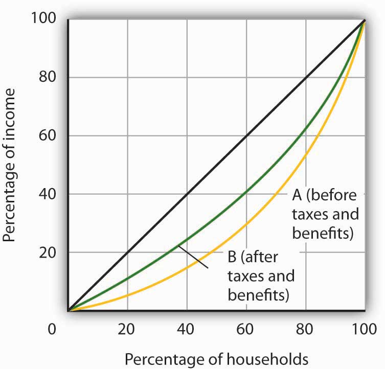
The accompanying Lorenz curves show the distribution of income in a country before taxes and welfare benefits are taken into account (curve A) and after taxes and welfare benefits are taken into account (curve B). Do taxes and benefits serve to make the distribution of income in the country more equal or more unequal?
In a fascinating examination of attitudes in the United States and in continental Western Europe, economists Alberto Alesina of Harvard University and George-Marios Angeletos of the Massachusetts Institute of Technology suggest that attitudes about the nature of income earning can lead to quite different economic systems and outcomes concerning the distribution of income.
The economists cite survey evidence from the World Values Survey, which concludes that 71% of Americans, and only 40% of Europeans, agree with the proposition: “The poor could become rich if they worked hard enough.” Further, Americans are much more likely to attribute material success to hard work, while Europeans tend to attribute success to factors such as luck, connections, and even corruption. The result, according to Professors Alesina and Angeletos, is that Americans select a government that is smaller and engages in less redistributive activity than is selected by Europeans. Government in continental Western Europe is 50% larger than in the United States, the tax system in Europe is much more progressive than in the United States, regulation of labor and product markets is more extensive in Europe, and redistributive programs are more extensive in Europe than in the United States. As a result, the income distribution in Europe is much more equal than in the United States.
People get what they expect. The economists derive two sets of equilibria. Equilibrium in a society in which people think incomes are a result of luck, connections, and corruption turns out to be precisely that. And, in a society in which people believe incomes are chiefly the result of effort and skill, they are. In the latter society, people work harder and invest more. In the United States, the average worker works 1,600 hours per year. In Europe, the average worker works 1,200 hours per year.
So, who is right—Americans with their “you get what you deserve” or Europeans with their “you get what luck, connections, and corruption bring you” attitude? The two economists show that people get, in effect, what they expect. European values and beliefs produce societies that are more egalitarian. American values and beliefs produce the American result: a society in which the distribution of income is more unequal, the government smaller, and redistribution relatively minor. Professors Alesina and Angeletos conclude that Europeans tend to underestimate the degree to which people can improve their material well-being through hard work, while Americans tend to overestimate that same phenomenon.
Source: Alberto Alesina and George-Marios Angeletos, “Fairness and Redistribution,” American Economic Review 95:4 (September, 2005) 960–80.
The Lorenz curve showing the distribution of income after taxes and benefits are taken into account is less bowed out than the Lorenz curve showing the distribution of income before taxes and benefits are taken into account. Thus, income is more equally distributed after taking them into account.
Poverty in the United States is something of a paradox. Per capita incomes in this country are among the highest on earth. Yet, the United States has a greater percentage of its population below the official poverty line than in the other industrialized nations. How can a nation that is so rich have so many people who are poor?
There is no single answer to the question of why so many people are poor. But we shall see that there are economic factors at work that help to explain poverty. We shall also examine the nature of the government’s response to poverty and the impact that response has. First, however, we shall examine the definition of poverty and look at some characteristics of the poor in the United States.
Suppose you were asked to determine whether a particular family was poor or not poor. How would you do it?
You might begin by listing the goods and services that would be needed to provide a minimum standard of living and then finding out if the family’s income was enough to purchase those items. If it were not, you might conclude that the family was poor. Alternatively, you might examine the family’s income relative to the incomes of other families in the community or in the nation. If the family was on the low end of the income scale, you might classify it as poor.
These two approaches represent two bases on which poverty is defined. The first is an absolute income testIncome test that sets a specific income level and defines a person as poor if his or her income falls below that level., which sets a specific income level and defines a person as poor if his or her income falls below that level. The second is a relative income testIncome test in which people whose incomes fall at the bottom of the income distribution are considered poor., in which people whose incomes fall at the bottom of the income distribution are considered poor. For example, we could rank households according to income as we did in the previous section on income inequality and define the lowest one-fifth of households as poor. In 2010, any U.S. household with an annual income below $20,000 fell in this category.
In contrast, to determine who is poor according to the absolute income test, we define a specific level of income, independent of how many households fall above or below it. The federal government defines a household as poor if the household’s annual income falls below a dollar figure called the poverty lineAmount of annual income below which the federal government defines a household as poor.. In 2010 the poverty line for a family of four was an income of $22,314. Figure 18.2 "Weighted Average Poverty Thresholds in 2010, by Size of Family" shows the poverty line for various family sizes.
Figure 18.2 Weighted Average Poverty Thresholds in 2010, by Size of Family
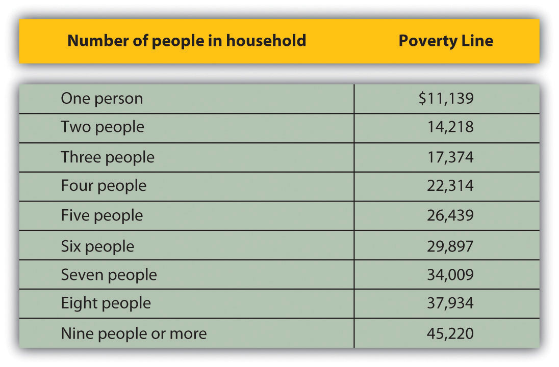
The Census Bureau uses a set of 48 money income thresholds that vary by family size and composition to determine who is in poverty. The “Weighted Average Poverty Thresholds” in the accompanying table is a summary of the 48 thresholds used by the census bureau. It provides a general sense of the “poverty line” based on the relative number of families by size and composition.
Source: DeNavas-Walt, Carmen, Bernadette D. Proctor, and Jessica Smith, U.S. Census Bureau, Current Population Reports, P60-239, Income, Poverty, and Health Insurance Coverage in the United States: 2010, U.S. Government Printing Office, Washington, D.C., 2011; p. 61.
The concept of a poverty line grew out of a Department of Agriculture study in 1955 that found families spending one-third of their incomes on food. With the one-third figure as a guide, the Department then selected food plans that met the minimum daily nutritional requirements established by the federal government. The cost of the least expensive plan for each household size was multiplied by three to determine the income below which a household would be considered poor. The government used this method to count the number of poor people from 1959 to 1969. The poverty line was adjusted each year as food prices changed. Beginning in 1969, the poverty line was adjusted annually by the average percentage price change for all consumer goods, not just changes in the price of food.
There is little to be said for this methodology for defining poverty. No attempt is made to establish an income at which a household could purchase basic necessities. Indeed, no attempt is made in the definition to establish what such necessities might be. The day has long passed when the average household devoted one-third of its income to food purchases; today such purchases account for less than one-seventh of household income. Still, it is useful to have some threshold that is consistent from one year to the next so that progress—or the lack thereof—in the fight against poverty can be assessed. In addition, the U.S. Census Bureau and the Bureau of Labor Statistics have begun working on more broad-based alternative measures of poverty. The new Supplemental Poverty Measure is based on expenses for food, clothing, shelter, and utilities; adjusts for geographic differences; adds in various in-kind benefits such as school lunches, housing subsidies, and energy assistance; includes tax credits; and then subtracts out taxes, work expenses, and out-of-pocket medical expenses.Kathleen Short, U.S. Census Bureau, Current Population Reports P60-241, Supplemental Poverty Measure: 2010, U.S. Government Printing Office, Washington, DC, November 2011.
The percentage of the population that falls below the poverty line is called the poverty rateThe percentage of the population that falls below the poverty line.. Figure 18.3 "The Poverty Rate in the United States, 1959–2010" shows both the number of people and the percentage of the population that fell below the poverty line each year since 1959.
Figure 18.3 The Poverty Rate in the United States, 1959–2010
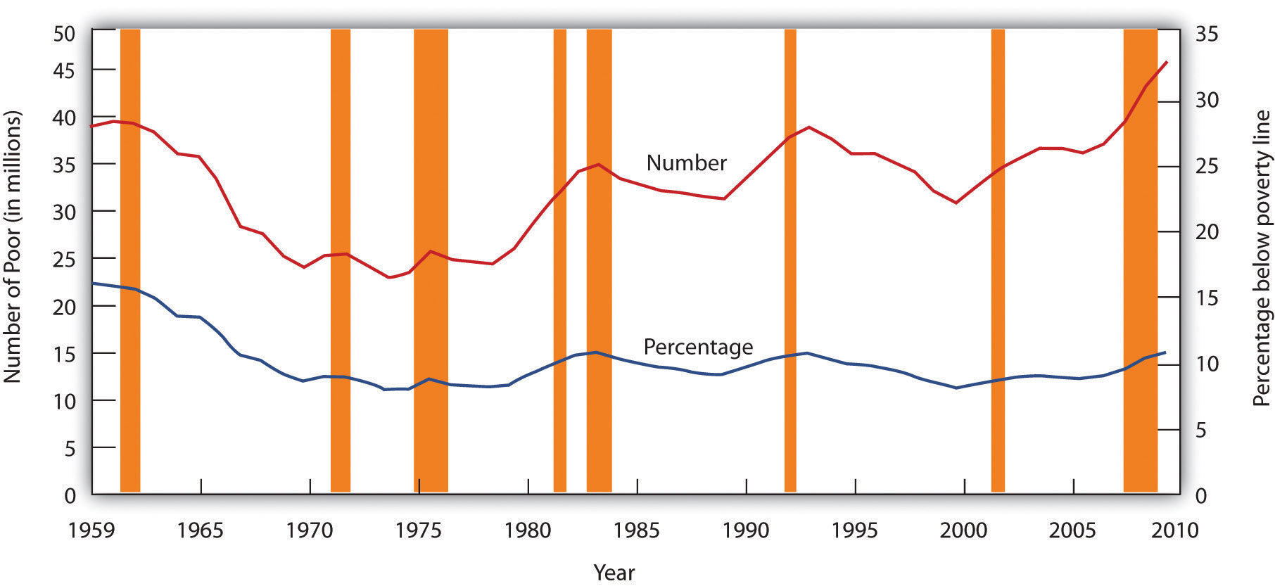
The curve shows the percentage of people who lived in households that fell below the poverty line in each year from 1959 to 2010. The poverty rate fell through the 1960s and since has been hovering between about 12% and 15%. It tends to rise during recessions.
Source: DeNavas-Walt, Carmen, Bernadette D. Proctor, and Jessica Smith, U.S. Census Bureau, Current Population Reports P60-239, Income, Poverty, and Health Insurance Coverage in the United States: 2010, U.S. Government Printing Office, Washington DC, 2011; Figure 4, p. 14.
Despite its shortcomings, measuring poverty using an absolute measure allows for the possibility of progress in reducing it; using a relative measure of poverty does not, since there will always be a lowest 1/5, or 1/10 of the population. But relative measures do make an important point: Poverty is in large measure a relative concept. In the United States, people defined as poor have much higher incomes than most of the world’s people or even than average Americans did as recently as the early 1970s. By international and historical standards, the average poor person in the United States is rich! The material possessions of America’s poor would be considered lavish in another time and in another place. For example, based on data from 2005 to 2009, 42% of poor households in the United States owned their own homes, nearly 75% owned a car, and 64% have cable or satellite TV. Over 80% of poor households had air conditioning. Forty years ago, only 36% of the entire population in the United States had air conditioning. The average poor person in the United States has more living space than the average person in London, Paris, Vienna, or Athens.Robert Rector and Rachel Sheffield, “Understanding Poverty in the United States: Surprising Facts about America’s Poor,” Heritage Foundation, Policy Research & Analysis, No. 2607, September 13, 2011.
We often think of poverty as meaning that poor people are unable to purchase adequate food. Yet, according to Department of Agriculture surveys, 83% of poor people report that they have adequate food and 96% of poor parents report that their children are never hungry because they cannot afford food. In short, poor people in the United States enjoy a standard of living that would be considered quite comfortable in many parts of the developed world—and lavish in the less developed world.Ibid.
But people judge their incomes relative to incomes of people around them, not relative to people everywhere on the planet or to people in years past. You may feel poor when you compare yourself to some of your classmates who may have fancier cars or better clothes. And a family of four in a Los Angeles slum with an annual income of $13,000 surely does not feel rich because its income is many times higher than the average family income in Ethiopia or of Americans of several decades ago. While the material possessions of poor Americans are vast by Ethiopian standards, they are low in comparison to how the average American lives. What we think of as poverty clearly depends more on what people around us are earning than on some absolute measure of income.
Both the absolute and relative income approaches are used in discussions of the poverty problem. When we speak of the number of poor people, we are typically using an absolute income test of poverty. When we speak of the problems of those at the bottom of the income distribution, we are speaking in terms of a relative income test. In the European Union, for example, the poverty line is set at 60% of the median income of each member nation in a particular year. That is an example of a relative measure of poverty. In the rest of this section, we focus on the absolute income test of poverty used in the United States.
There is no iron law of poverty that dictates that a household with certain characteristics will be poor. Nonetheless, poverty is much more highly concentrated among some groups than among others. The six characteristics of families that are important for describing who in the United States constitute the poor are whether or not the family is headed by a female, age, the level of education, whether or not the head of the family is working, the race of the household, and geography.
Figure 18.4 "The Demographics of Poverty in the United States, 2010" shows poverty rates for various groups and for the population as a whole in 2010. What does it tell us?
The incidence of poverty soars when several of these demographic factors associated with poverty are combined. For example, the poverty rate for families with children that are headed by women who lack a high school education is higher than 50%.
The new, more broad-based Supplemental Poverty Measure shows an increase of only 0.1 compared to the official poverty rate measure, but bigger differences for different segments of the population. For example, a smaller percentage of people under the age of 18 are poor according to the supplemental poverty measure (18.2% versus 22.5%), while a larger percentage of those over 64 years of age are considered poor (15.9% versus 9.0%). The new measure also shows lower poverty rates among blacks, renters, people living outside metropolitan areas, and those covered by only public health insurance. Other groups show the same or higher poverty rates.Kathleen Short, U.S. Census Bureau, Current Population Reports P60-241, Supplemental Poverty Measure: 2010, U.S. Government Printing Office, Washington, DC, November 2011.
Figure 18.4 The Demographics of Poverty in the United States, 2010
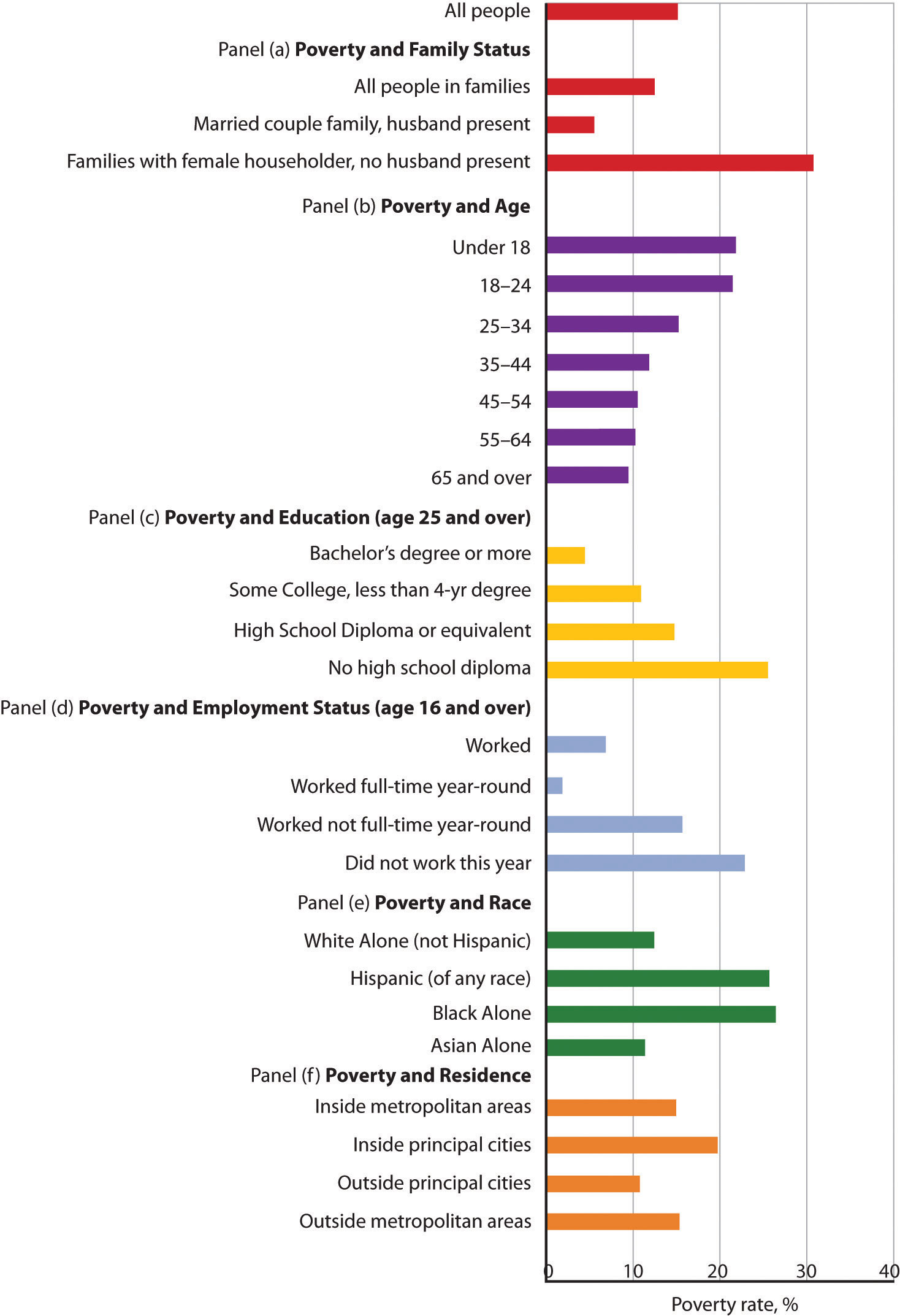
Poverty rates in the United States vary significantly according to a variety of demographic factors. Panels (a) through (f) compare poverty rates among different groups of the U.S. population. The data are for 2010.
Source: DeNavas-Walt, Carmen, Bernadette D. Proctor, and Jessica C. Smith, U.S. Census Bureau, Current Population Reports, P60-239, Income, Poverty, and Health Insurance Coverage: 2010, U.S. Government Printing Office, Washington DC, 2011. Data for educational attainment, employment status, and residence from the Annual Social and Economic Supplement 2010, poverty tables at http://www.census.gov/hhes/www/cpstables/032011/pov/toc.htm.
Consider a young single parent with three small children. The parent is not employed and has no support from other relatives. What does the government provide for the family?
The primary form of cash assistance is likely to come from a program called Temporary Assistance for Needy Families (TANF). This program began with the passage of the Personal Responsibility and Work Opportunity Reconciliation Act of 1996. It replaced Aid to Families with Dependent Children (AFDC). TANF is funded by the federal government but administered through the states. Eligibility is limited to two years of continuous payments and to five years in a person’s lifetime, although 20% of a state’s caseload may be exempted from this requirement.
In addition to this assistance, the family is likely to qualify for food stamps, which are vouchers that can be exchanged for food at the grocery store. The family may also receive rent vouchers, which can be used as payment for private housing. The family may qualify for Medicaid, a program that pays for physician and hospital care as well as for prescription drugs.
A host of other programs provide help ranging from counseling in nutrition to job placement services. The parent may qualify for federal assistance in attending college. The children may participate in the Head Start program, a program of preschool education designed primarily for low-income children. If the poverty rate in the area is unusually high, local public schools the children attend may receive extra federal aid. Welfare programsThe array of programs that government provides to alleviate poverty. are the array of programs that government provides to alleviate poverty.
In addition to public sector support, a wide range of help is available from private sector charities. These may provide scholarships for education, employment assistance, and other aid.
Figure 18.5 "Welfare Programs and the Poor" shows participation rates in the major federal programs to help the poor.
Figure 18.5 Welfare Programs and the Poor
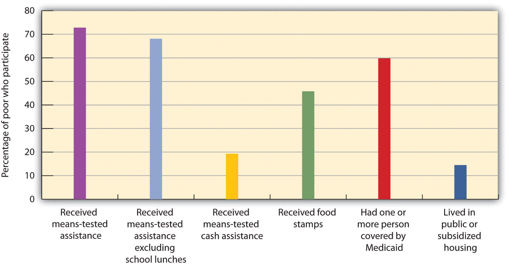
Many people who fall below the poverty line have not received aid from particular programs.
Source: U.S. Census Bureau, Current Population Survey, 2010 Annual Social and Economic Supplement.
Not all people whose incomes fall below the poverty line received aid. In 2010, a substantial majority of those counted as poor received some form of aid. However, as shown in Figure 18.5 "Welfare Programs and the Poor", the percentages who were helped by individual programs were much lower. Less than 20% of people below the poverty line received some form of cash assistance in 2010. About 45% received food stamps and nearly 60% lived in a household in which one or more people received medical services through Medicaid. Only about one-seventh of the people living in poverty received some form of housing aid.
Although for the most part poverty programs are federally funded, individual states set eligibility standards and administer the programs. Allowing states to establish their own programs was a hallmark feature of the 1996 welfare reform. As state budgets have come under greater pressure, many states have tightened standards.
Aid provided to people falls into two broad categories: cash and noncash assistance. Cash assistanceA money payment that an aid recipient can spend as he or she wishes. is a money payment that a recipient can spend as he or she wishes. Noncash assistanceThe provision of specific goods and services, such as food or medical services, job training, or subsidized child care rather than cash. is the provision of specific goods and services, such as food or medical services, job training, or subsidized child care rather than cash.
Noncash assistance is the most important form of aid to the poor. The large share of noncash relative to cash assistance raises two issues. First, since the poor would be better off (that is, reach a higher level of satisfaction) with cash rather than noncash assistance, why is noncash aid such a large percentage of total aid to the poor? Second, the importance of noncash assistance raises an important issue concerning the methodology by which the poverty rate is measured in the United States. We examine these issues in turn.
Why Noncash Aid?
Suppose you had a choice between receiving $515 or a television set worth $515. Neither gift is taxable. Which would you take?
Given a choice between cash and an equivalent value in merchandise, you would probably take the cash. Unless the television set happened to be exactly what you would purchase with the $515, you could find some other set of goods and services that you would prefer to the TV set. The same is true of funds that you can spend on anything versus funds whose spending is restricted. Given a choice of $515 that you could spend on anything and $515 that you could spend only on food, which would you choose? A given pool of funds allows consumers a greater degree of satisfaction than does a specific set of goods and services.
We can conclude that poor people who receive government aid would be better off from their own perspectives with cash grants than with noncash aid. Why, then, is most government aid given as noncash benefits?
Economists have suggested two explanations. The first is based on the preferences of donors. Recipients might prefer cash, but the preferences of donors matter also. The donors, in this case, are taxpayers. Suppose they want poor people to have specific things—perhaps food, housing, and medical care.
Given such donor preferences, it is not surprising to find aid targeted at providing these basic goods and services. A second explanation has to do with the political clout of the poor. The poor are not likely to be successful competitors in the contest to be at the receiving end of public sector income redistribution efforts; most redistribution goes to people who are not poor. But firms that provide services such as housing or medical care might be highly effective lobbyists for programs that increase the demand for their products. They could be expected to seek more help for the poor in the form of noncash aid that increases their own demand and profits.Students who have studied rent seeking behavior will recognize this argument. It falls within the public choice perspective of public finance theory.
Poverty Management and Noncash Aid
Only cash income is counted in determining the official poverty rate. The value of food, medical care, or housing provided through various noncash assistance programs is not included in household income. That is an important omission, because most government aid is noncash aid. Data for the official poverty rate thus do not reflect the full extent to which government programs act to reduce poverty.
The Census Bureau estimates the impact of noncash assistance on poverty. If a typical household would prefer, say, $515 in cash to $515 in food stamps, then $515 worth of food stamps is not valued at $515 in cash. Economists at the Census Bureau adjust the value of noncash aid downward to reflect an estimate of its lesser value to households. Suppose, for example, that given the choice between $515 in food stamps and $475 in cash, a household reports that it is indifferent between the two—either would be equally satisfactory. That implies that $515 in food stamps generates satisfaction equal to $475 in cash; the food stamps are thus “worth” $475 to the household.
The welfare system in the United States came under increasing attack in the 1980s and early 1990s. It was perceived to be expensive, and it had clearly failed to eliminate poverty. Many observers worried that welfare was becoming a way of life for people who had withdrawn from the labor force, and that existing welfare programs did not provide an incentive for people to work. President Clinton made welfare reform one of the key issues in the 1992 presidential campaign.
The Personal Responsibility and Work Opportunity Reconciliation Act of 1996 was designed to move people from welfare to work. It eliminated the entitlement aspect of welfare by defining a maximum period of eligibility. It gave states considerable scope in designing their own programs. In the first years following welfare reform, the number of people on welfare dropped by several million. Much research on the impact of reform showed that caseloads declined and employment increased and that the law did not have an adverse effect on poverty or the well-being of children. This positive outcome seemed to have resulted from an expansion of the earned income tax credit that also occurred, the overall low unemployment rate until the most recent few years, and larger behavioral responses than had been expected.Marianne P. Bitler and Hilary W. Hoynes, “The State of the Social Safety Net in the Post-Welfare Reform Era,” Brookings Papers on Economic Activity (Fall 2010): 71–127.
Advocates of welfare reform proclaimed victory, while critics pointed to the booming economy, the tight labor market, and the general increase in the number of jobs over the same period. The recession that began at the end of 2007 and the ensuing slow recovery in the unemployment rate provided a real-time test of the effects of the reform. Economists Marianne Bitler and Hilary Hoynes analyzed the impact of welfare reform during the Great Recession on nonelderly families with children. They found that participation in cash assistance programs seemed less responsive to the downturn but that participation in noncash safety net programs, particularly the food stamp program, had become more responsive. They did find some evidence that the increase in poverty or near-poverty status might have been greater than it would have been without the reform.Marianne P. Bitler and Hilary W. Hoynes, “The State of the Social Safety Net in the Post-Welfare Reform Era,” Brookings Papers on Economic Activity (Fall 2010): 71–127.
Just as the increase in income inequality begs for explanation, so does the question of why poverty seems so persistent. Should not the long periods of economic growth in the 1980s and 1990s and from 2003 to late 2007 have substantially reduced poverty? Have the various government programs been ineffective?
Clearly, some of the same factors that have contributed to rising income inequality have also contributed to the persistence of poverty. In particular, the increases in households headed by females and the growing gaps in wages between skilled and unskilled workers have been major contributors.
Tax policy changes have reduced the extent of poverty. In addition to general reductions in tax rates, the Earned Income Tax Credit, which began in 1975 and was expanded in the 1990s, provides people below a certain income level with a supplement for each dollar of income earned. This supplement, roughly 30 cents for every dollar earned, is received as a tax refund at the end of the year.
Figure 18.6 Percentages of Population in Eight Countries with Disposable Incomes Less Than 1/2 the National Median
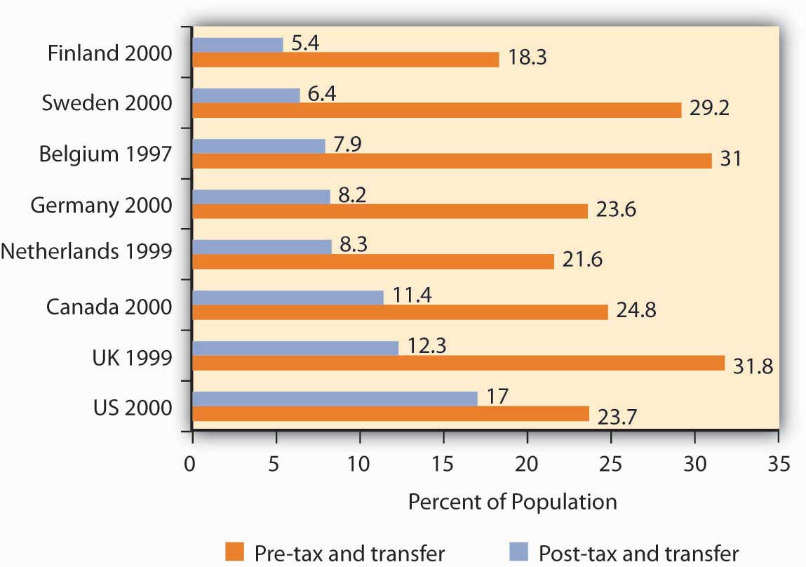
Source: Timothy M. Smeeding, “Public Policy, Economic Inequality, and Poverty: The United States in Comparative Perspectives,” Social Science Quarterly, 86 (December 2005): 955–983.
Taken together, though, transfer payment and tax programs in the United States are less effective in reducing poverty than are the programs of other developed countries. Figure 18.6 "Percentages of Population in Eight Countries with Disposable Incomes Less Than 1/2 the National Median" shows the percentage of the population in eight developed countries with a disposable income (income after taxes) less than one-half the national median. The figure shows this percentage both before and after tax and transfer payment programs are considered. Clearly, the United States is the least aggressive in seeking to eliminate poverty among the eight countries shown.
How does poverty relate to work? Look back at Figure 18.4 "The Demographics of Poverty in the United States, 2010". Many of the poor are children or adults over age 65 and some are already working full time. Taken together, these three groups represent more than half of those in poverty. Also included amongst the poor are people who are ill or disabled, people who do not work due to family or home reasons, and people who are in school. The Census Bureau found in 2010 that of the nation’s 46.2 million poor people, nearly 3 million reported they were not working or worked only part of the year or part time because they could not find full-time work.Current Population Survey, Annual Social and Economic Supplement 2010, Table POV24. So, while more employment opportunities would partly alleviate poverty, reducing unemployment is clearly only part of the answer.
How effective have government programs been in alleviating poverty? The Census Bureau’s supplemental poverty measure begins to answer that question. For example, those calculations show a reduction of two percentage points in the poverty rate, from 18% to 16%, when the earned income tax credit is included, ceteris paribus. Inclusion of the Supplemental Nutritional Assistance Program reduced the poverty rate by 1.7%, and housing subsidies reduced it by 0.9%. Other programs each had smaller effects on poverty reduction. But it is also important to distinguish between the poverty rate and the degree of poverty. Cash programs might reduce the degree of poverty but might not affect a family’s income enough to actually move that family above the poverty line. Thus, even though the gap between the family’s income and the poverty line is lessened, the family is still classified as poor and would thus still be included in the poverty-rate figures.
The Smiths, a family of four, have an income of $20,500 in 2006. Using the absolute income test approach and the data given in the chapter, determine if this family is poor. Use the relative income test to determine if this family is poor.
The governments of the United States and of Great Britain have taken sharply different courses in their welfare reform efforts. In the United States, the primary reform effort was undertaken in 1996, with the declaration to eliminate welfare as an entitlement and the beginning of programs that required recipients to enter the labor force within two years. President Clinton promised to “end welfare as we know it.”
In Britain, the government of Tony Blair took a radically different approach. Prime Minister Blair promised to “make welfare popular again.” His government undertook to establish what he called a “third way” to welfare reform, one that emphasized returning recipients to the workforce but that also sought explicitly to end child poverty.
The British program required recipients to get counseling aimed at encouraging them to return to the labor force. It did not, however, require that they obtain jobs. It also included a program of “making work pay,” the primary feature of which was the creation of a National Minimum Wage, one that was set higher than the minimum wage in the United States. In the United States, the minimum wage equaled 34% of median private sector wages in 2002; the British minimum wage was set at 45% of the median private sector wage in 2002.
The British program, which was called the New Deal, featured tax benefits for poor families with children, whether they worked or not. It also included a Sure Start program of child care for poor people with children under three years old. In short, the Blair program was a more extensive social welfare program than the 1996 act in the United States.
The table below compares results of the two programs in terms of their impact on child poverty, using an “absolute” poverty line and also using a relative poverty line.
| Child Poverty Rates, Pre- and Post- Reform | ||
|---|---|---|
| United Kingdom | Absolute (percent) | Relative (percent) |
| 1997–1998 | 24 | 25 |
| 2002–2003 | 12 | 21 |
| Change | −12 | −4 |
| United States | Absolute (percent) | Relative (percent) |
| 1992 | 19 | 38 |
| 2001 | 13 | 35 |
| Change | −6 | −3 |
| Child Poverty Rates in Single-Mother Families, Pre- and Post- Reform | ||
|---|---|---|
| United Kingdom | Absolute (percent) | Relative (percent) |
| 1997–1998 | 40 | 41 |
| 2002–2003 | 15 | 33 |
| Change | −25 | −8 |
| United States | Absolute (percent) | Relative (percent) |
| 1992 | 44 | 67 |
| 2001 | 28 | 59 |
| Change | −16 | −8 |
The relative measure of child poverty is the method of measuring poverty adopted by the European Union. It draws the poverty line at 60% of median income. The poverty line is thus a moving target against which it is more difficult to make progress.
Hills and Waldfogel compared the British results to those in the United States in terms of the relative impact on welfare caseloads, employment of women having families, and reduction in child poverty. They note that reduction in welfare caseloads was much greater in the United States, with caseloads falling from 5.5 million to 2.3 million. In Britain, the reduction in caseloads was much smaller. In terms of impact on employment among women, the United States again experienced a much more significant increase. In terms of reduction of child poverty, however, the British approach clearly achieved a greater reduction. The British approach also increased incomes of families in the bottom 10% of the income distribution (i.e., the bottom decile) by more than that achieved in the United States. In Britain, incomes of families in the bottom decile rose 22%, and for families with children they rose 24%. In the United States, those in the bottom decile had more modest gains.
Would the United States ever adopt a New Deal program such as the Blair program in Great Britain? That, according to Hills and Waldfogel, would require a change in attitudes in the United States that they regard as unlikely.
Source: John Hills and Jane Waldfogel, “A ‘Third Way’ in Welfare Reform? Evidence from the United Kingdom,” Journal of Policy Analysis and Management, 23(4) (2004): 765–88.
According to the absolute income test, the Smiths are poor because their income of $20,500 falls below the 2006 poverty threshold of $20,614. According to the relative income test, they are not poor because their $20,500 income is above the upper limit of the lowest quintile, $20,035.
We have seen that being a female head of household or being a member of a racial minority increases the likelihood of being at the low end of the income distribution and of being poor. In the real world, we know that on average women and members of racial minorities receive different wages from white male workers, even though they may have similar qualifications and backgrounds. They might be charged different prices or denied employment opportunities. This section examines the economic forces that create such discrimination, as well as the measures that can be used to address it.
DiscriminationWhen people with similar economic characteristics experience different economic outcomes because of their race, sex, or other noneconomic characteristics. occurs when people with similar economic characteristics experience different economic outcomes because of their race, sex, or other noneconomic characteristics. A black worker whose skills and experience are identical to those of a white worker but who receives a lower wage is a victim of discrimination. A woman denied a job opportunity solely on the basis of her gender is the victim of discrimination. To the extent that discrimination exists, a country will not be allocating resources efficiently; the economy will be operating inside its production possibilities curve.
Pioneering work on the economics of discrimination was done by Gary S. Becker, an economist at the University of Chicago, who won the Nobel Prize in economics in 1992. He suggested that discrimination occurs because of people’s preferences or attitudes. If enough people have prejudices against certain racial groups, or against women, or against people with any particular characteristic, the market will respond to those preferences.
In Becker’s model, discriminatory preferences drive a wedge between the outcomes experienced by different groups. Discriminatory preferences can make salespeople less willing to sell to one group than to another or make consumers less willing to buy from the members of one group than from another or to make workers of one race or sex or ethnic group less willing to work with those of another race, sex, or ethnic group.
Let us explore Becker’s model by examining labor-market discrimination against black workers. We begin by assuming that no discriminatory preferences or attitudes exist. For simplicity, suppose that the supply curves of black and white workers are identical; they are shown as a single curve in Figure 18.7 "Prejudice and Discrimination". Suppose further that all workers have identical marginal products; they are equally productive. In the absence of racial preferences, the demand for workers of both races would be D. Black and white workers would each receive a wage W per unit of labor. A total of L black workers and L white workers would be employed.
Figure 18.7 Prejudice and Discrimination
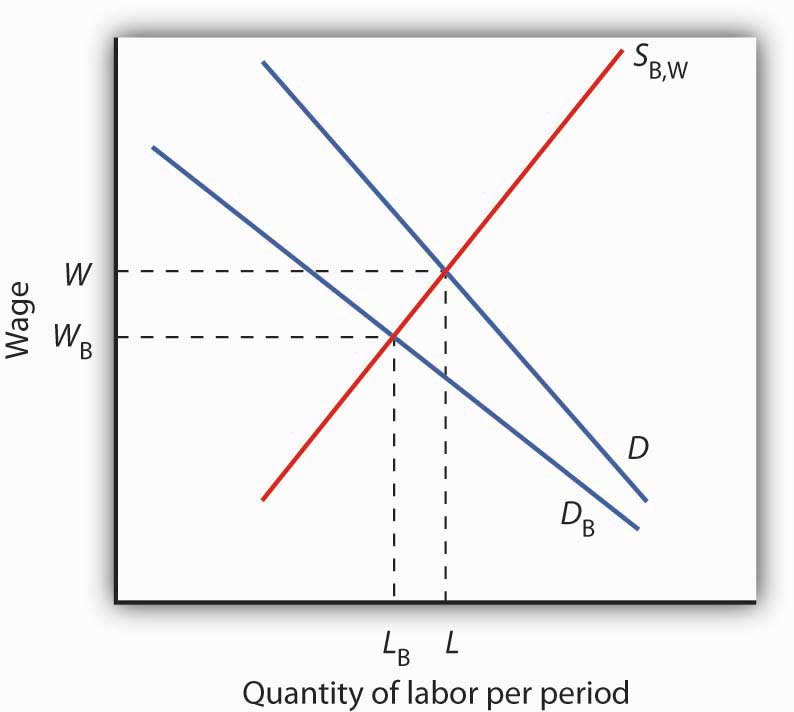
If employers, customers, or employees have discriminatory preferences, and those preferences are widespread, then the marketplace will result in discrimination. Here, black workers receive a lower wage and fewer of them are employed than would be the case in the absence of discriminatory preferences.
Now suppose that employers have discriminatory attitudes that cause them to assume that a black worker is less productive than an otherwise similar white worker. Now employers have a lower demand, DB, for black than for white workers. Employers pay black workers a lower wage, WB, and employ fewer of them, LB instead of L, than they would in the absence of discrimination.
As illustrated in Figure 18.7 "Prejudice and Discrimination", racial prejudices on the part of employers produce discrimination against black workers, who receive lower wages and have fewer employment opportunities than white workers. Discrimination can result from prejudices among other groups in the economy as well.
One source of discriminatory prejudices is other workers. Suppose, for example, that white workers prefer not to work with black workers and require a wage premium for doing so. Such preferences would, in effect, raise the cost to the firm of hiring black workers. Firms would respond by demanding fewer of them, and wages for black workers would fall.
Another source of discrimination against black workers could come from customers. If the buyers of a firm’s product prefer not to deal with black employees, the firm might respond by demanding fewer of them. In effect, prejudice on the part of consumers would lower the revenue that firms can generate from the output of black workers.
Whether discriminatory preferences exist among employers, employees, or consumers, the impact on the group discriminated against will be the same. Fewer members of that group will be employed, and their wages will be lower than the wages of other workers whose skills and experience are otherwise similar.
Race and sex are not the only characteristics that affect hiring and wages. Some studies have found that people who are short, overweight, or physically unattractive also suffer from discrimination, and charges of discrimination have been voiced by disabled people and by homosexuals. Whenever discrimination occurs, it implies that employers, workers, or customers have discriminatory preferences. For the effects of such preferences to be felt in the marketplace, they must be widely shared.
There are, however, market pressures that can serve to lessen discrimination. For example, if some employers hold discriminatory preferences but others do not, it will be profit enhancing for those who do not to hire workers from the group being discriminated against. Because workers from this group are less expensive to hire, costs for non-discriminating firms will be lower. If the market is at least somewhat competitive, firms who continue to discriminate may be driven out of business.
Reacting to demands for social change brought on most notably by the civil rights and women’s movements, the federal government took action against discrimination. In 1954, the U.S. Supreme Court rendered its decision that so-called separate but equal schools for black and white children were inherently unequal, and the Court ordered that racially segregated schools be integrated. The Equal Pay Act of 1963 requires employers to pay the same wages to men and women who do substantially the same work. Federal legislation was passed in 1965 to ensure that minorities were not denied the right to vote.
Congress passed the most important federal legislation against discrimination in 1964. The Civil Rights Act barred discrimination on the basis of race, sex, or ethnicity in pay, promotion, hiring, firing, and training. An Executive Order issued by President Lyndon Johnson in 1967 required federal contractors to implement affirmative action programs to ensure that members of minority groups and women were given equal opportunities in employment. The practical effect of the order was to require that these employers increase the percentage of women and minorities in their work forces. Affirmative action programs for minorities followed at most colleges and universities.
What has been the outcome of these efforts to reduce discrimination? A starting point is to look at wage differences among different groups. Gaps in wages between males and females and between blacks and whites have fallen over time. In 1955, the wages of black men were about 60% of those of white men; in 2010, they were 74% of those of white men. For black men, the reduction in the wage gap occurred primarily between 1965 and 1973. In contrast, the gap between the wages of black women and white men closed more substantially, and progress in closing the gap continued after 1973, albeit at a slower rate. Specifically, the wages of black women were about 35% of those of white men in 1955, 58% in 1975, and 70% in 2010. For white women, the pattern of gain is still different. The wages of white women were about 65% of those of white men in 1955 and fell to about 60% from the mid-1960s to the late 1970s. The wages of white females relative to white males have improved, however, over the last 40 years. In 2010, white female wages were 80% of white male wages. While there has been improvement in wage gaps between black men, black women, and white women vis-à-vis white men, a substantial gap still remains. Figure 18.8 "The Wage Gap" shows the wage differences for the period 1969–2010.
Figure 18.8 The Wage Gap
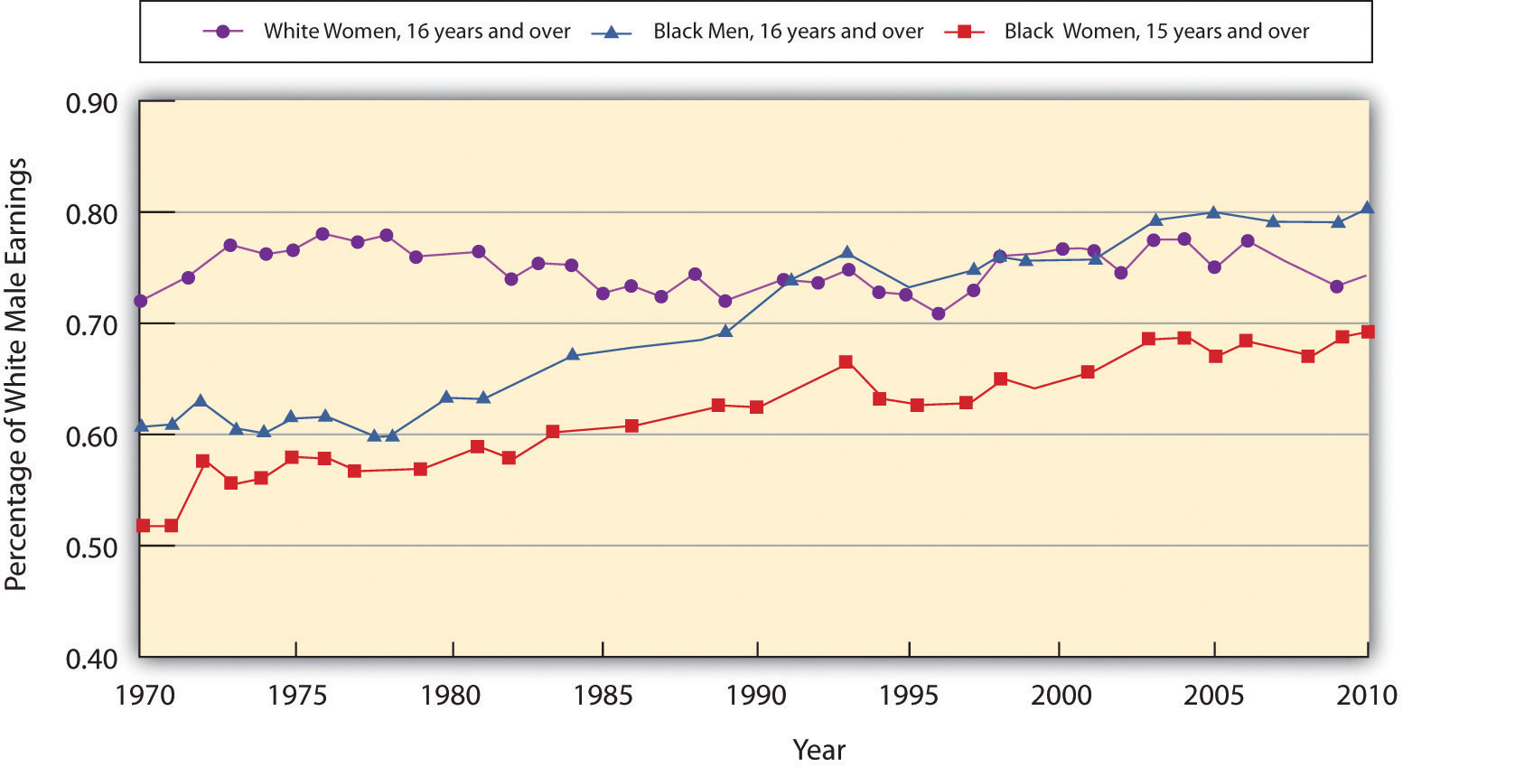
The exhibit shows the wages of white women, black women, and black men as a percentage of the wages of white men from 1969–2010. As you can see, the gap has closed considerably, but there remains a substantial gap between the wages of white men and those of other groups in the economy. Part of the difference is a result of discrimination.
Source: Table 37. Median weekly earnings of full-time wage and salary workers, by selected characteristics. For recent years, http://www.bls.gov/cps/tables.htm.
One question that economists try to answer is the extent to which the gaps are due to discrimination per se and the extent to which they reflect other factors, such as differences in education, job experience, or choices that individuals in particular groups make about labor-force participation. Once these factors are accounted for, the amount of the remaining wage differential due to discrimination is less than the raw differentials presented in Figure 18.8 "The Wage Gap" would seem to indicate.
There is evidence as well that the wage differential due to discrimination against women and blacks, as measured by empirical studies, has declined over time. For example, a number of studies have concluded that black men in the 1980s and 1990s experienced a 12 to 15% loss in earnings due to labor-market discrimination.William A. Darity and Patrick L. Mason, “Evidence on Discrimination in Employment,” Journal of Economic Perspectives 12:2 (Spring 1998): 63–90. University of Chicago economist James Heckman denies that the entire 12% to 15% differential is due to racial discrimination, pointing to problems inherent in measuring and comparing human capital among individuals. Nevertheless, he reports that the earnings loss due to discrimination similarly measured would have been between 30 and 40% in 1940 and still over 20% in 1970.James J. Heckman, “Detecting Discrimination,” Journal of Economic Perspectives 12:2 (Spring 1998): 101–16.
Can civil rights legislation take credit for the reductions in labor-market discrimination over time? To some extent, yes. A study by Heckman and John J. Donohue III, a law professor at Northwestern University, concluded that the landmark 1964 Civil Rights Act, as well as other civil rights activity leading up to the act, had the greatest positive impact on blacks in the South during the decade following its passage. Evidence of wage gains by black men in other regions of the country was, however, minimal. Most federal activity was directed toward the South, and the civil rights effort shattered an entire way of life that had subjugated black Americans and had separated them from mainstream life.John J. Donohue III and James Heckman, “Continuous Versus Episodic Change: The Impact of Civil Rights Policy on the Economic Status of Blacks,” Journal of Economic Literature 29 (December 1991): 1603–43.
In recent years, affirmative action programs have been under attack. Proposition 209, passed in California in 1996, and Initiative 200, passed in Washington State in 1998, bar preferential treatment due to race in admission to public colleges and universities in those states. The 1996 Hopwood case against the University of Texas, decided by the United States Court of Appeals for the Fifth Circuit, eliminated the use of race in university admissions, both public and private, in Texas, Louisiana, and Mississippi. Then Supreme Court decisions in 2003 concerning the use of affirmative action at the University of Michigan upheld race conscious admissions, so long as applicants are still considered individually and decisions are based on multiple criteria.
Controversial research by two former Ivy League university presidents, political scientist Derek Bok of Harvard University and economist William G. Bowen of Princeton University, concluded that affirmative action policies have created the backbone of the black middle class and taught white students the value of integration. The study focused on affirmative action at 28 elite colleges and universities. It found that while blacks enter those institutions with lower test scores and grades than those of whites, receive lower grades, and graduate at a lower rate, after graduation blacks earn advanced degrees at rates identical to those of their former white classmates and are more active in civic affairs.Derek Bok and William G. Bowen, The Shape of the River: Long-Term Consequences of Considering Race in College and University Admissions (Princeton, N. J.: Princeton University Press, 1998).
While stricter enforcement of civil rights laws or new programs designed to reduce labor-market discrimination may serve to further improve earnings of groups that have been historically discriminated against, wage gaps between groups also reflect differences in choices and in “premarket” conditions, such as family environment and early education. Some of these premarket conditions may themselves be the result of discrimination.
The narrowing in wage differentials may reflect the dynamics of the Becker model at work. As people’s preferences change, or are forced to change due to competitive forces and changes in the legal environment, discrimination against various groups will decrease. However, it may be a long time before discrimination disappears from the labor market, not only due to remaining discriminatory preferences but also because the human capital and work characteristics that people bring to the labor market are decades in the making. The election of Barack Obama as president of the United States in 2008 is certainly a hallmark in the long and continued struggle against discrimination.
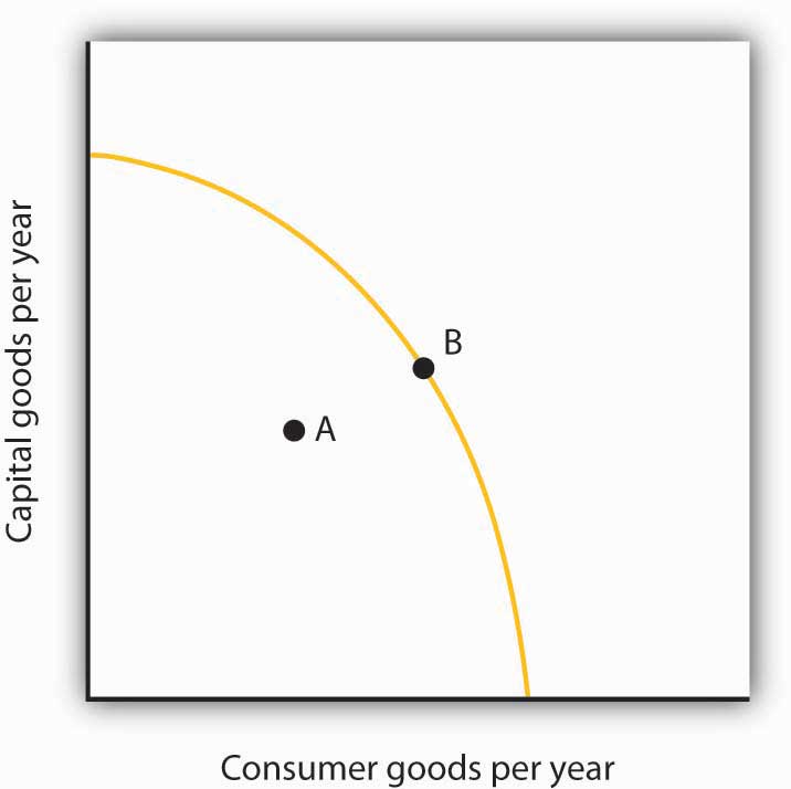
Use a production possibilities curve to illustrate the impact of discrimination on the production of goods and services in the economy. Label the horizontal axis as consumer goods per year. Label the vertical axis as capital goods per year. Label a point A that shows an illustrative bundle of the two which can be produced given the existence of discrimination. Label another point B that lies on the production possibilities curve above and to the right of point A. Use these two points to describe the outcome that might be expected if discrimination were eliminated.
Many authors have pointed out that differences in “pre-market” conditions may drive observed differences in market outcomes for people in different groups. Significant inroads to the reduction of poverty may lie in improving the educational opportunities available to minority children and others living in poverty-level households, but at what point in their lives is the pay-off to intervention the largest? Professor James Heckman, in an op-ed essay in The Wall Street Journal, argues that the key to improving student performance and adult competency lies in early intervention in education.
Professor Heckman notes that spending on children after they are already in school has little impact on their later success. Reducing class sizes, for example, does not appear to promote gains in factors such as attending college or earning higher incomes. What does seem to matter is earlier intervention. By the age of eight , differences in learning abilities are essentially fixed. But, early intervention to improve cognitive and especially non-cognitive abilities (the latter include qualities such as perseverance, motivation, and self-restraint) has been shown to produce significant benefits. In an experiment begun several decades ago known as the Perry intervention, four-year-old children from disadvantaged homes were given programs designed to improve their chances for success in school. Evaluations of the program 40 years later found that it had a 15 to 17% rate of return in terms of the higher wages earned by men and women who had participated in the program compared to those from similar backgrounds who did not—the program’s benefit-cost ratio was 8 to 1. Professor Heckman argues that even earlier intervention among disadvantaged groups would be desirable—perhaps as early as six months of age.
Economists Rob Grunewald and Art Rolnick of the Federal Reserve Bank of Minneapolis have gone so far as to argue that, because of the high returns to early childhood development programs, which they estimate at 12% per year to the public, state and local governments, can promote more economic development in their areas by supporting early childhood programs than they currently do by offering public subsidies to attract new businesses to their locales or to build new sports stadiums, none of which offers the prospects of such a high rate of return.
Sources: James Heckman, “Catch ’em Young,” The Wall Street Journal, January 10, 2006, p. A-14; Rob Grunewald and Art Rolnick, “Early Childhood Development on a Large Scale,” Federal Reserve Bank of Minneapolis The Region, June 2005.
Discrimination leads to an inefficient allocation of resources and results in production levels that lie inside the production possibilities curve (PPC) (point A). If discrimination were eliminated, the economy could increase production to a point on the PPC, such as B.
In this chapter, we looked at three issues related to the question of fairness: income inequality, poverty, and discrimination.
The distribution of income in the United States has become more unequal in the last four decades. Among the factors contributing to increased inequality have been changes in family structure, technological change, and tax policy. While rising inequality can be a concern, there is a good deal of movement of families up and down the distribution of income, though recently mobility may have decreased somewhat.
Poverty can be measured using an absolute or a relative income standard. The official measure of poverty in the United States relies on an absolute standard. This measure tends to overstate the poverty rate because it does not count noncash welfare aid as income. The new supplemental poverty measures have begun to take these programs into account. Poverty is concentrated among female-headed households, minorities, people with relatively little education, and people who are not in the labor force. Children have a particularly high poverty rate.
Welfare reform in 1996 focused on moving people off welfare and into work. It limits the number of years that individuals can receive welfare payments and allows states to design the specific parameters of their own welfare programs. Following the reform, the number of people on welfare fell dramatically. The long-term impact on poverty is still under investigation.
Federal legislation bans discrimination. Affirmative action programs, though controversial, are designed to enhance opportunities for minorities and women. Wage gaps between women and white males and between blacks and white males have declined since the 1950s. For black males, however, most of the reduction occurred between 1965 and 1973. Much of the decrease in wage gaps is due to acquisition of human capital by women and blacks, but some of the decrease also reflects a reduction in discrimination.
Discuss the advantages and disadvantages of the following three alternatives for dealing with the rising inequality of wages.
Here are income distribution data for three countries, from the Human Development Report 2005, table 15. Note that here we report only four data points rather than the five associated with each quintile. These emphasize the distribution at the extremes of the distribution.
| Poorest 10% | Poorest 20% | Richest 20% | Richest 10% | |
|---|---|---|---|---|
| Panama | 0.7 | 2.4 | 60.3 | 43.3 |
| Sweden | 3.6 | 9.1 | 36.6 | 22.2 |
| Singapore | 1.9 | 5.0 | 49.0 | 32.8 |
Looking at Figure 18.7 "Prejudice and Discrimination" suppose the wage that black workers are receiving in a discriminatory environment, WB, is $25 per hour, while the wage that white workers receive, W, is $30 per hour. Now suppose a regulation is imposed that requires that black workers be paid $30 per hour also.
Suppose the poverty line in the United States was set according to the test required in the European Union: a household is poor if its income is less than 60% of the median household income. Here are annual data for median household income in the United States for the period 1994–2004. The data also give the percentage of the households that fall below 60% of the median household income.
Source: U.S Census Bureau, Current Population Reports, P60-229; Income in 2004 CPI-U-RS adjusted dollars; column 3 estimated by authors using Table A-1, p. 31.
| Median Household Income in the U.S. | Percent of households with income below 60% of median | |
|---|---|---|
| 1994 | 40,677 | 30.1 |
| 1995 | 41,943 | 30.4 |
| 1996 | 42,544 | 29.9 |
| 1997 | 43,430 | 29.1 |
| 1998 | 45,003 | 27.8 |
| 1999 | 46,129 | 27.1 |
| 2000 | 46,058 | 26.4 |
| 2001 | 45,062 | 27.4 |
| 2002 | 44,546 | 27.8 |
| 2003 | 44,482 | 28.3 |
| 2004 | 44,389 | 28.3 |
Consider the following model of the labor market in the United States. Suppose that the labor market consists of two parts, a market for skilled workers and the market for unskilled workers, with different demand and supply curves for each as given below. The initial wage for skilled workers is $20 per hour; the initial wage for unskilled workers is $7 per hour.


