Large Sample Estimation of a Population Mean

7.1 Large Sample Estimation of a Population Mean

Learning Objectives

To become familiar with the concept of an interval estimate of the population mean.
To understand how to apply formulas for a confidence interval for a population mean.

The Central Limit Theorem says that, for large samples (samples of size n ≥ 30), when viewed as a random variable the sample mean $\bar{X}$ is normally distributed with mean $μ_{\bar{X}} = μ$ and standard deviation $σ_{\bar{X}} = σ ∕ \sqrt{n} .$ The Empirical Rule says that we must go about two standard deviations from the mean to capture 95% of the values of $\bar{X}$ generated by sample after sample. A more precise distance based on the normality of $\bar{X}$ is 1.960 standard deviations, which is $E = 1.960 σ ∕ \sqrt{n} .$

The key idea in the construction of the 95% confidence interval is this, as illustrated in Figure 7.1 "When Winged Dots Capture the Population Mean": because in sample after sample 95% of the values of $\bar{X}$ lie in the interval $[μ - E, μ + E]$ , if we adjoin to each side of the point estimate $\bar{x}$ a “wing” of length E, 95% of the intervals formed by the winged dots contain μ. The 95% confidence interval is thus $\bar{x} \pm 1.960 σ ∕ \sqrt{n} .$ For a different level of confidenceThe proportion of confidence intervals which, if under repeated random sampling were always constructed according to the formula of the text, would contain the parameter of interest., say 90% or 99%, the number 1.960 will change, but the idea is the same.

Figure 7.1 When Winged Dots Capture the Population Mean

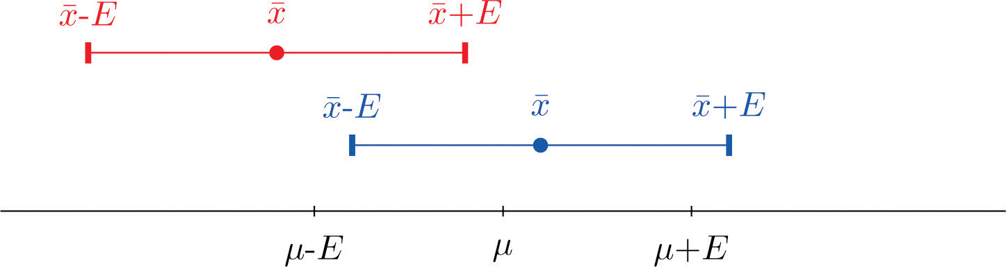
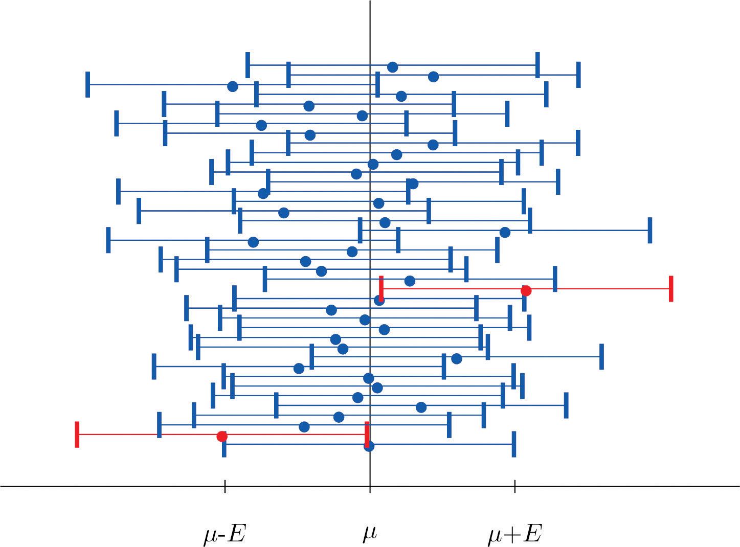
Figure 7.2 "Computer Simulation of 40 95% Confidence Intervals for a Mean" shows the intervals generated by a computer simulation of drawing 40 samples from a normally distributed population and constructing the 95% confidence interval for each one. We expect that about $(0.05) (40) = 2$ of the intervals so constructed would fail to contain the population mean μ, and in this simulation two of the intervals, shown in red, do.

Figure 7.2 Computer Simulation of 40 95% Confidence Intervals for a Mean

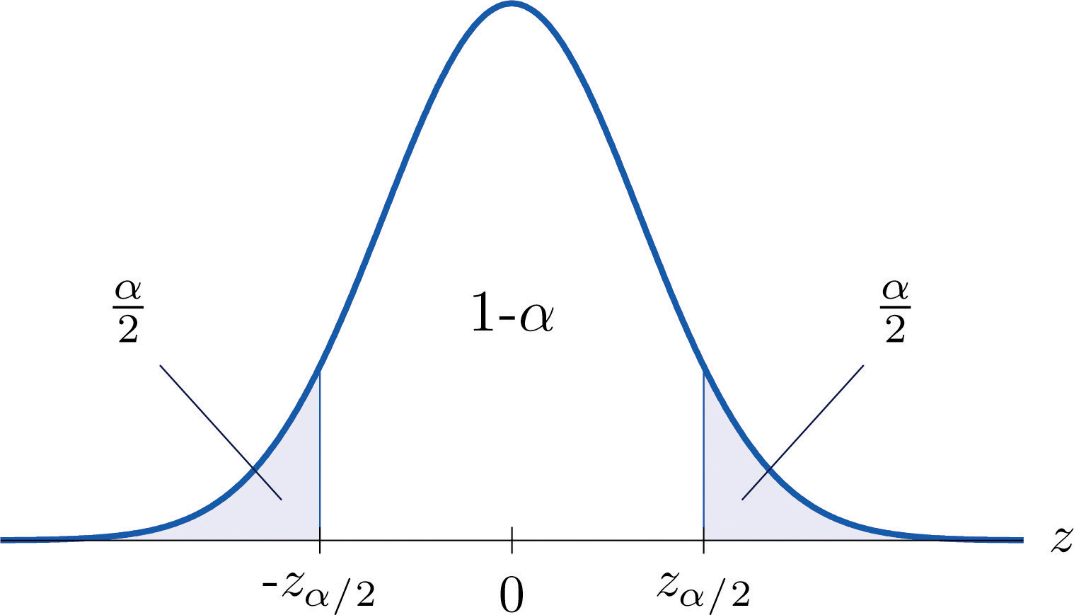
It is standard practice to identify the level of confidence in terms of the area $α$ in the two tails of the distribution of $\bar{X}$ when the middle part specified by the level of confidence is taken out. This is shown in Figure 7.3, drawn for the general situation, and in Figure 7.4, drawn for 95% confidence. Remember from Section 5.4.1 "Tails of the Standard Normal Distribution" in Chapter 5 "Continuous Random Variables" that the z-value that cuts off a right tail of area c is denoted z_c. Thus the number 1.960 in the example is $z_{. 025}$ , which is $z_{α ∕ 2}$ for $α = 1 - 0.95 = 0.05 .$

Figure 7.3

For $100 (1 - α)$ % confidence the area in each tail is $α ∕ 2 .$

Figure 7.4

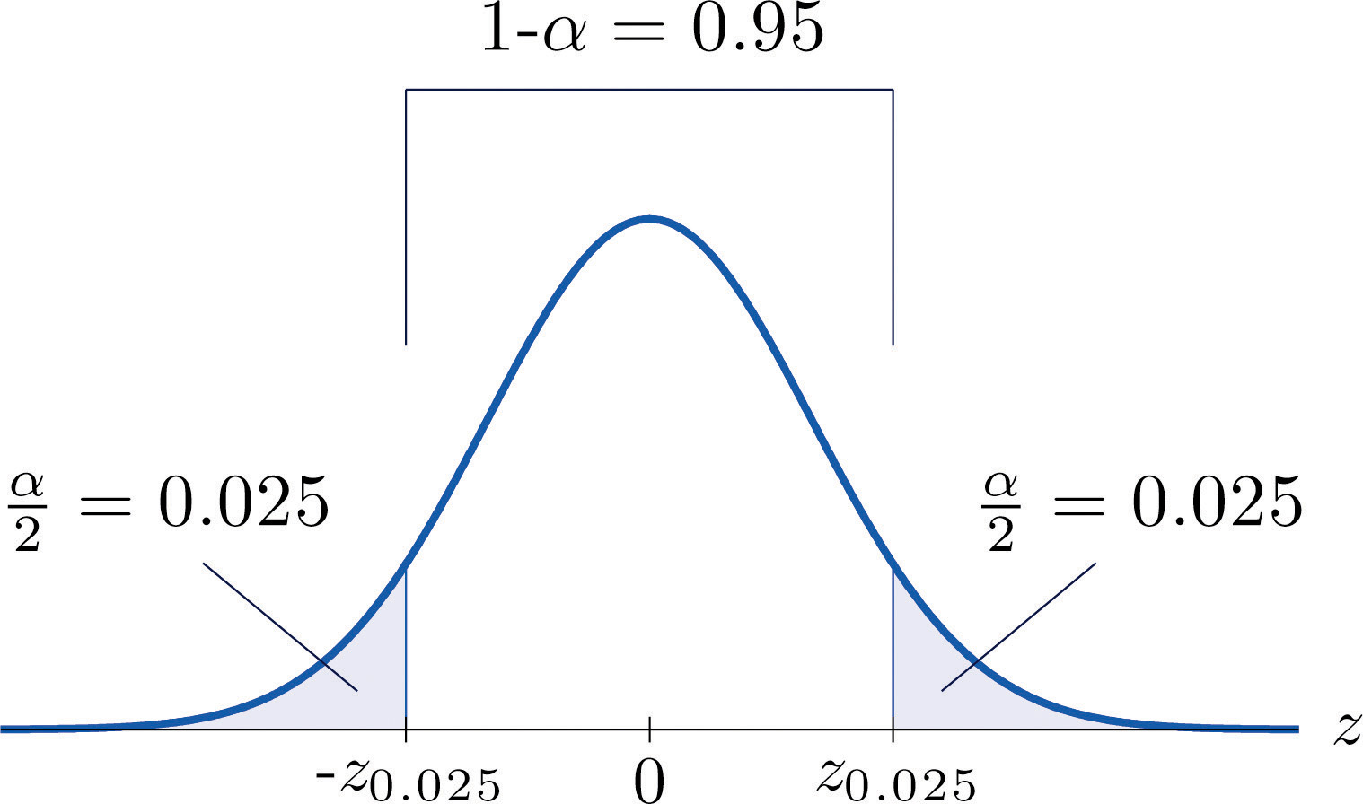
For 95% confidence the area in each tail is $α ∕ 2 = 0.025 .$

The level of confidence can be any number between 0 and 100%, but the most common values are probably 90% ( $α = 0.10$ ), 95% ( $α = 0.05$ ), and 99% ( $α = 0.01$ ).

Thus in general for a $100 (1 - α)$ % confidence interval, $E = z_{α ∕ 2} (σ ∕ \sqrt{n})$ , so the formula for the confidence interval is $\bar{x} \pm z_{α ∕ 2} (σ ∕ \sqrt{n}) .$ While sometimes the population standard deviation σ is known, typically it is not. If not, for n ≥ 30 it is generally safe to approximate σ by the sample standard deviation s.

Large Sample $100 (1 - α) %$ Confidence Interval for a Population Mean

If σ is known: $\bar{x} \pm z_{α ∕ 2} (\frac{σ}{\sqrt{n}})$

If σ is unknown: $\bar{x} \pm z_{α ∕ 2} (\frac{s}{\sqrt{n}})$

A sample is considered large when n ≥ 30.

As mentioned earlier, the number $E = z_{α ∕ 2} σ ∕ \sqrt{n}$ or $E = z_{α ∕ 2} s ∕ \sqrt{n}$ is called the margin of error of the estimate.

Example 1

Find the number $z_{α ∕ 2}$ needed in construction of a confidence interval:

when the level of confidence is 90%;
when the level of confidence is 99%.

Solution:

For confidence level 90%, $α = 1 - 0.90 = 0.10$ , so $z_{α ∕ 2} = z_{0.05} .$ The procedure for finding this number was given in Section 5.4.1 "Tails of the Standard Normal Distribution". Since the area under the standard normal curve to the right of $z_{. 05}$ is 0.05, the area to the left of z_0.05 is 0.95. We search for the area 0.9500 in Figure 12.2 "Cumulative Normal Probability". The closest entries in the table are 0.9495 and 0.9505, corresponding to z-values 1.64 and 1.65. Since 0.95 is exactly halfway between 0.9495 and 0.9505 we use the average 1.645 of the z-values for z_0.05.
For confidence level 99%, $α = 1 - 0.99 = 0.01$ , so $z_{α ∕ 2} = z_{0.005} .$ Since the area under the standard normal curve to the right of z_0.005 is 0.005, the area to the left of z_0.005 is 0.9950. We search for the area 0.9950 in Figure 12.2 "Cumulative Normal Probability". The closest entries in the table are 0.9949 and 0.9951, corresponding to z-values 2.57 and 2.58. Since 0.995 is halfway between 0.9949 and 0.9951 we use the average 2.575 of the z-values for z_0.005.

Example 2

Use Figure 12.3 "Critical Values of " to find the number $z_{α ∕ 2}$ needed in construction of a confidence interval:

when the level of confidence is 90%;
when the level of confidence is 99%.

Solution:

In the next section we will learn about a continuous random variable that has a probability distribution called the Student t-distribution. Figure 12.3 "Critical Values of " gives the value t_c that cuts off a right tail of area c for different values of c. The last line of that table, the one whose heading is the symbol $\infty$ for infinity and $[z]$ , gives the corresponding z-value z_c that cuts off a right tail of the same area c. In particular, z_0.05 is the number in that row and in the column with the heading t_0.05. We read off directly that $z_{0.05} = 1.645 .$
In Figure 12.3 "Critical Values of " z_0.005 is the number in the last row and in the column headed t_0.005, namely 2.576.

Figure 12.3 "Critical Values of " can be used to find z_c only for those values of c for which there is a column with the heading t_c appearing in the table; otherwise we must use Figure 12.2 "Cumulative Normal Probability" in reverse. But when it can be done it is both faster and more accurate to use the last line of Figure 12.3 "Critical Values of " to find z_c than it is to do so using Figure 12.2 "Cumulative Normal Probability" in reverse.

Example 3

A sample of size 49 has sample mean 35 and sample standard deviation 14. Construct a 98% confidence interval for the population mean using this information. Interpret its meaning.

Solution:

For confidence level 98%, $α = 1 - 0.98 = 0.02$ , so $z_{α ∕ 2} = z_{0.01} .$ From Figure 12.3 "Critical Values of " we read directly that $z_{0.01} = 2.326 .$ Thus

\bar{x} \pm z_{α ∕ 2} \frac{s}{\sqrt{n}} = 35 \pm 2.326 (\frac{14}{\sqrt{49}}) = 35 \pm 4.652 \approx 35 \pm 4.7

We are 98% confident that the population mean μ lies in the interval $[30 . 3,39 . 7]$ , in the sense that in repeated sampling 98% of all intervals constructed from the sample data in this manner will contain μ.

Example 4

A random sample of 120 students from a large university yields mean GPA 2.71 with sample standard deviation 0.51. Construct a 90% confidence interval for the mean GPA of all students at the university.

Solution:

For confidence level 90%, $α = 1 - 0.90 = 0.10$ , so $z_{α ∕ 2} = z_{0.05} .$ From Figure 12.3 "Critical Values of " we read directly that $z_{0.05} = 1.645 .$ Since n = 120, $\bar{x} = 2.71$ , and s = 0.51,

\bar{x} \pm z_{α ∕ 2} \frac{s}{\sqrt{n}} = 2.71 \pm 1.645 (\frac{0.51}{\sqrt{120}}) = 2.71 \pm 0.0766

One may be 90% confident that the true average GPA of all students at the university is contained in the interval $(2.71 - 0 . 08,2 . 71 + 0.08) = (2 . 63,2 . 79) .$

Key Takeaways

A confidence interval for a population mean is an estimate of the population mean together with an indication of reliability.
There are different formulas for a confidence interval based on the sample size and whether or not the population standard deviation is known.
The confidence intervals are constructed entirely from the sample data (or sample data and the population standard deviation, when it is known).

Exercises

Basic

A random sample is drawn from a population of known standard deviation 11.3. Construct a 90% confidence interval for the population mean based on the information given (not all of the information given need be used).
1. n = 36, $\bar{x} = 105.2$ , s = 11.2
2. n = 100, $\bar{x} = 105.2$ , s = 11.2
A random sample is drawn from a population of known standard deviation 22.1. Construct a 95% confidence interval for the population mean based on the information given (not all of the information given need be used).
1. n = 121, $\bar{x} = 82.4$ , s = 21.9
2. n = 81, $\bar{x} = 82.4$ , s = 21.9
A random sample is drawn from a population of unknown standard deviation. Construct a 99% confidence interval for the population mean based on the information given.
1. n = 49, $\bar{x} = 17.1$ , s = 2.1
2. n = 169, $\bar{x} = 17.1$ , s = 2.1
A random sample is drawn from a population of unknown standard deviation. Construct a 98% confidence interval for the population mean based on the information given.
1. n = 225, $\bar{x} = 92.0$ , s = 8.4
2. n = 64, $\bar{x} = 92.0$ , s = 8.4
A random sample of size 144 is drawn from a population whose distribution, mean, and standard deviation are all unknown. The summary statistics are $\bar{x} = 58.2$ and s = 2.6.
1. Construct an 80% confidence interval for the population mean μ.
2. Construct a 90% confidence interval for the population mean μ.
3. Comment on why one interval is longer than the other.
A random sample of size 256 is drawn from a population whose distribution, mean, and standard deviation are all unknown. The summary statistics are $\bar{x} = 1011$ and s = 34.
1. Construct a 90% confidence interval for the population mean μ.
2. Construct a 99% confidence interval for the population mean μ.
3. Comment on why one interval is longer than the other.

Applications

A government agency was charged by the legislature with estimating the length of time it takes citizens to fill out various forms. Two hundred randomly selected adults were timed as they filled out a particular form. The times required had mean 12.8 minutes with standard deviation 1.7 minutes. Construct a 90% confidence interval for the mean time taken for all adults to fill out this form.
Four hundred randomly selected working adults in a certain state, including those who worked at home, were asked the distance from their home to their workplace. The average distance was 8.84 miles with standard deviation 2.70 miles. Construct a 99% confidence interval for the mean distance from home to work for all residents of this state.
On every passenger vehicle that it tests an automotive magazine measures, at true speed 55 mph, the difference between the true speed of the vehicle and the speed indicated by the speedometer. For 36 vehicles tested the mean difference was −1.2 mph with standard deviation 0.2 mph. Construct a 90% confidence interval for the mean difference between true speed and indicated speed for all vehicles.
A corporation monitors time spent by office workers browsing the web on their computers instead of working. In a sample of computer records of 50 workers, the average amount of time spent browsing in an eight-hour work day was 27.8 minutes with standard deviation 8.2 minutes. Construct a 99.5% confidence interval for the mean time spent by all office workers in browsing the web in an eight-hour day.
A sample of 250 workers aged 16 and older produced an average length of time with the current employer (“job tenure”) of 4.4 years with standard deviation 3.8 years. Construct a 99.9% confidence interval for the mean job tenure of all workers aged 16 or older.
The amount of a particular biochemical substance related to bone breakdown was measured in 30 healthy women. The sample mean and standard deviation were 3.3 nanograms per milliliter (ng/mL) and 1.4 ng/mL. Construct an 80% confidence interval for the mean level of this substance in all healthy women.
A corporation that owns apartment complexes wishes to estimate the average length of time residents remain in the same apartment before moving out. A sample of 150 rental contracts gave a mean length of occupancy of 3.7 years with standard deviation 1.2 years. Construct a 95% confidence interval for the mean length of occupancy of apartments owned by this corporation.
The designer of a garbage truck that lifts roll-out containers must estimate the mean weight the truck will lift at each collection point. A random sample of 325 containers of garbage on current collection routes yielded $\bar{x} = 75.3$ lb, s = 12.8 lb. Construct a 99.8% confidence interval for the mean weight the trucks must lift each time.
In order to estimate the mean amount of damage sustained by vehicles when a deer is struck, an insurance company examined the records of 50 such occurrences, and obtained a sample mean of $2,785 with sample standard deviation $221. Construct a 95% confidence interval for the mean amount of damage in all such accidents.
In order to estimate the mean FICO credit score of its members, a credit union samples the scores of 95 members, and obtains a sample mean of 738.2 with sample standard deviation 64.2. Construct a 99% confidence interval for the mean FICO score of all of its members.

Additional Exercises

For all settings a packing machine delivers a precise amount of liquid; the amount dispensed always has standard deviation 0.07 ounce. To calibrate the machine its setting is fixed and it is operated 50 times. The mean amount delivered is 6.02 ounces with sample standard deviation 0.04 ounce. Construct a 99.5% confidence interval for the mean amount delivered at this setting. Hint: Not all the information provided is needed.
A power wrench used on an assembly line applies a precise, preset amount of torque; the torque applied has standard deviation 0.73 foot-pound at every torque setting. To check that the wrench is operating within specifications it is used to tighten 100 fasteners. The mean torque applied is 36.95 foot-pounds with sample standard deviation 0.62 foot-pound. Construct a 99.9% confidence interval for the mean amount of torque applied by the wrench at this setting. Hint: Not all the information provided is needed.
The number of trips to a grocery store per week was recorded for a randomly selected collection of households, with the results shown in the table.
$\begin{matrix} 2 & 2 & 2 & 1 & 4 & 2 & 3 & 2 & 5 & 4 \\ 2 & 3 & 5 & 0 & 3 & 2 & 3 & 1 & 4 & 3 \\ 3 & 2 & 1 & 6 & 2 & 3 & 3 & 2 & 4 & 4 \end{matrix}$
Construct a 95% confidence interval for the average number of trips to a grocery store per week of all households.
For each of 40 high school students in one county the number of days absent from school in the previous year were counted, with the results shown in the frequency table.
$\begin{matrix} x & 0 & 1 & 2 & 3 & 4 & 5 \\ f & 24 & 7 & 5 & 2 & 1 & 1 \end{matrix}$
Construct a 90% confidence interval for the average number of days absent from school of all students in the county.
A town council commissioned a random sample of 85 households to estimate the number of four-wheel vehicles per household in the town. The results are shown in the following frequency table.
$\begin{matrix} x & 0 & 1 & 2 & 3 & 4 & 5 \\ f & 1 & 16 & 28 & 22 & 12 & 6 \end{matrix}$
Construct a 98% confidence interval for the average number of four-wheel vehicles per household in the town.
The number of hours per day that a television set was operating was recorded for a randomly selected collection of households, with the results shown in the table.
$\begin{matrix} 3.7 & 4.2 & 1.5 & 3.6 & 5.9 \\ 4.7 & 8.2 & 3.9 & 2.5 & 4.4 \\ 2.1 & 3.6 & 1.1 & 7.3 & 4.2 \\ 3.0 & 3.8 & 2.2 & 4.2 & 3.8 \\ 4.3 & 2.1 & 2.4 & 6.0 & 3.7 \\ 2.5 & 1.3 & 2.8 & 3.0 & 5.6 \end{matrix}$
Construct a 99.8% confidence interval for the mean number of hours that a television set is in operation in all households.

Large Data Set Exercises

Large Data Set 1 records the SAT scores of 1,000 students. Regarding it as a random sample of all high school students, use it to construct a 99% confidence interval for the mean SAT score of all students.

http://www.gone.2012books.lardbucket.org/sites/all/files/data1.xls
Large Data Set 1 records the GPAs of 1,000 college students. Regarding it as a random sample of all college students, use it to construct a 95% confidence interval for the mean GPA of all students.

http://www.gone.2012books.lardbucket.org/sites/all/files/data1.xls
Large Data Set 1 lists the SAT scores of 1,000 students.

http://www.gone.2012books.lardbucket.org/sites/all/files/data1.xls
1. Regard the data as arising from a census of all students at a high school, in which the SAT score of every student was measured. Compute the population mean μ.
2. Regard the first 36 students as a random sample and use it to construct a 99% confidence for the mean μ of all 1,000 SAT scores. Does it actually capture the mean μ?
Large Data Set 1 lists the GPAs of 1,000 students.

http://www.gone.2012books.lardbucket.org/sites/all/files/data1.xls
1. Regard the data as arising from a census of all freshman at a small college at the end of their first academic year of college study, in which the GPA of every such person was measured. Compute the population mean μ.
2. Regard the first 36 students as a random sample and use it to construct a 95% confidence for the mean μ of all 1,000 GPAs. Does it actually capture the mean μ?

Answers

1. $105.2 \pm 3.10$
2. $105.2 \pm 1.86$
1. $17.1 \pm 0.77$
2. $17.1 \pm 0.42$
1. $58.2 \pm 0.28$
2. $58.2 \pm 0.36$
3. Asking for greater confidence requires a longer interval.

$12.8 \pm 0.20$
$− 1.2 \pm 0.05$
$4.4 \pm 0.79$
$3.7 \pm 0.19$
$2785 \pm 61$

$6.02 \pm 0.03$
$2.8 \pm 0.48$
$2.54 \pm 0.30$

$(1511 . 43,1546 . 05)$
1. μ = 1528.74
2. $(1428 . 22,1602 . 89)$

7.1 Large Sample Estimation of a Population Mean

Learning Objectives

Large Sample 100(1−α)% Confidence Interval for a Population Mean

Example 1

Example 2

Example 3

Example 4

Key Takeaways

Exercises

Basic

Applications

Additional Exercises

Large Data Set Exercises

Answers

Large Sample $100 (1 - α) %$ Confidence Interval for a Population Mean